Building Time-Specific Population Grid Models for Urban Planning
This presentation discusses the importance of time-specific population models for urban planning, utilizing data from various sources to create grid models for daytime population estimates. Examples, methodologies, and data sources are explored in detail.

Building Time-Specific Population Grid Models for Urban Planning
E N D
Presentation Transcript
Building time-specific population grid models David Martin, University of Southampton, UK EFGS, 5 October 2009
Acknowledgements • Samantha Cockings and Samuel Leung • Economic and Social Research Council award number RES-062-23-1811 • Employee data from the Annual Business Inquiry Service, National Online Manpower Information Service, licence NTC/ABI07-P3020. Office for National Statistics 2001 Census: Standard Area Statistics (England and Wales): ESRC Census Programme, Census Dissemination Unit, Mimas (University of Manchester). National Statistics Postcode Directory Data: Office for National Statistics, Postcode Directories: ESRC Census Programme, Census Geography Data Unit (UKBORDERS), EDINA (University of Edinburgh). Quarterly Labour Force Survey, Economic and Social Data Service, usage number 40023.
Presentation overview • Introduction • Space-time population modelling • Data sources • Modelling framework • Early results and conclusion
Introduction • Importance of small area population mapping • Advantages of gridded population models: esp. stability over time and reconstruction of settlement geography • Deficiencies of current “night-time approaches” • Enormous growth of new population-related data sources
(Schmitt, 1956, p. 83). • “One of the most important and difficult problems now facing city planners is the development of accurate, usable techniques for estimating the current daytime population of census tracts in urban areas” • Why? Reasons included modelling the location and size of bomb shelters and the potential casualties resulting from a nuclear attack • Schmitt, R. C. (1956) Estimating Daytime Populations. Journal of the American Planning Association 22 (2), 83-85
Space-time population modelling • ~99% of work based on night-time; ~0.5% daytime? • Numerous motivations for time-specific models: emergency planning, transportation, business location, etc. • General approach is to start with night-time population map and transfer population subgroups to specific daytime locations, e.g. schools, workplaces • Longstanding difficulty of obtaining data with sufficient space/time resolution • In reality, many different timescales to be modelled
Examples • Emergency response in US cities – Sleeter and Wood (2006) • US hazard exposure and response – McPherson et al. (2006) • Landscan USA - Bhadhuri et al. (2007) • Helsinki - Ahola et al. (2007) • UK Health and Safety Executive – Smith and Fairburn (2008)
http://www.ornl.gov/sci/gist/landscan/landscanUSA/landscanUSA_factsheet_ORNL.pdfhttp://www.ornl.gov/sci/gist/landscan/landscanUSA/landscanUSA_factsheet_ORNL.pdf
Data sources - residential • Census- or register-based, using “usual place of residence” • Residence definition – equivalent to night-time population locations, students counted at term-time residence • Decennial update interval – long-term population change • UK census at output area level (OA, pop ~300) and official mid-year estimates (MYEs) at Lower Super OA level (LSOA, pop ~1500) • Some workplace data from census, but not all people have workplaces and not all workplaces are daytime locations
Data sources – non-residential • New administrative sources esp. from government, Neighbourhood Statistics Service (NeSS) • Huge growth in availability and frequency since 2001 census • Annual Business Inquiry dataset (employers, employees) • Schools, hospitals, visitor attractions, long-distance visitor numbers, transportation flows • Indirect measures of retail, leisure activity, points of interest • Can all be related to NeSS geography hierarchy, NSPD
Mapping population to activities/places… Residential Private dwellings Communal ests. Education Employment Temp accomm. Healthcare Total population +/- external visitors ...and further subdivisions Non-residential Family/social Retail Leisure Tourism Generalized local Road Rail Transport Metro/subway Air Water
What do current maps cover? Residential Private dwellings Census, MYE Communal ests. Census, MYE Education Employment Temp accomm. Healthcare Total population +/- external visitors Non-residential Family/social Retail Leisure Tourism Generalized local Road Rail Transport Metro/subway Air Water
Residential Private dwellings Census, MYE Communal ests. Census, MYE Education NeSS, EduBase Employment Census, ABI, QLFS Temp accomm. VisitBritain, ABI Healthcare Total population +/- external visitors HES Non-residential Family/social VisitBritain Retail ABI, commercial Leisure DCMS, ALVA, etc. Tourism DCMS, ALVA, etc. Generalized local Road DfT, AADF Rail National Rail Transport Metro/subway TfL, etc Air CAA Water TfL Data sources for all non-residential ID2007, NeSS
Modelling framework • Builds on Martin (1989, 2006), Martin et al. (2000) currently implemented in SurfaceBuilder program • One of a variety of methods for reallocation of population counts onto a series of geographical features • Akin to dasymetric models where known population counts are allocated to most likely set of spatial locations • Adaptive kernel estimation, treating each centroid as a high information point. • Weight each cell to receive population reallocated from local centroids, hence volume preserving
Centroids, boundaries and grids Left: centroid locations and boundaries; Right: centroid populations redistributed onto grid
Distance decay function Always try to provide a caption next to your picture in this style
Extension to the spatio-temporal problem • Spatial centroid: • Population count • Spatial extent • Time-space centroid: • Population capacity • Spatial extent • Time profile • Area of influence • e.g. census output area • Census population • Modelled • e.g. primary school • Pupil numbers • Small (one cell) • Term dates, school day • Catchment area (modelled time/space)
Time profile example – school Population In transit Present 00 06 12 18 00 Time of day
Treatment of centroid i at time t centroid i background layer b local extent d area of influence j study area a
Background layer • Population “capacity” • Land use • Land cover • Pop density • Transport
Basic time-space interpolation algorithm • Specify study area a and time t • Identify background layer b (cells that can contain population) for time t • Adjust for external visitors in/out of a at time t • Sum all residential centroids to obtain population P • Examine each centroid i to obtain populations p in local extent d and area of influence j at time t • Redistribute P across d and j, constrained by b
Early results • Southampton, UK as test area • Using existing model with pre-prepared data extracts for specific time slices (SurfaceBuilder program) • Does not require full time profiles for each centroid • Does not take background layer into account, hence no population is allocated into transport layer • Time-space interpolation program currently being written in .Net using existing and new code components • Preliminary validation against known patterns
02:00 Southampton, 200m cells Residential “night-time” model 28
08:00 Southampton, 200m cells Early workplaces, docks, industrial estates; rest as residential 29
09:00 Southampton, 200m cells Workplaces, educational institutions, “daytime” model; low residential; very high central densities 30
18:00 Southampton, 200m cells Late workplaces remain, education closed; return to residential; high central densities 31
Initial visualization of output Output to kml Multiple layers overlaid in Google Earth 3D navigation and exploration Time slider allows time sequence to be “played” 32

