Multiple Linear Regression: Introduction
In this session, you'll learn to interpret results from multiple linear regression models with more than one explanatory variable. You will explore hypotheses tested by parameter estimates and t-values while addressing outliers identified via residual plots. Through real-life examples like child mortality and household poverty, this session equips you to analyze the impact of various factors. A practical case study involving university students will illustrate how age, college years, and parental income affect perceptions of crime, boosting your analytical skills in regression analysis.


Multiple Linear Regression: Introduction
E N D
Presentation Transcript
Multiple Linear Regression: Introduction (Session 06)
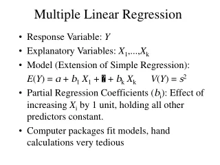
Learning Objectives At the end of this session, you will be able to • interpret results from a regression model with more than one explanatory variable • understand the specific hypotheses being tested by t-values associated with parameter estimates • have an appreciation of what might be done with outliers, identified via residual plots
More than one explanatory variable In real life examples, the following type of questions may be asked… • What factors affect child mortality? • Can household socio-economic characteristics be identified that relate closely to household poverty levels? • Would provision of free fertiliser and packs of seed increase crop productivity and hence improved livelihoods of farmers? Addressing these leads to fitting multiple linear regression models
Example with 3 explanatory variables A random sample of 45 university students were asked to personally decide which of a set of 25 acts they would consider to be a crime. The number of acts selected was recorded as the variable named “crimes”. Data were also collected on each student’s age, years in college and income of parents. Question: Which of the three factors (if any) have an effect on students’ views on what acts constitute crime?
Start with some scatter plots crimes age Parents’ income College years y = number of acts regarded as being criminal x1 = age x2 = years in college x3 = parents’ income
Initial visual impression • Crimes appears most strongly associated with age and income, although for age, this association is not linear – also one outlier? • Crimes does not appear associated with years in college • Can test whether these observations are telling us something real about the relationship by regression analysis procedures
Aim Would aim for the simplest possible model • i.e. one with fewest parameters • that still adequately summarises the relationship of response (here crimes) and one or more of the predictors (here age, college years, and income) • and gives information on which of the explanatory variables make a contribution to variability in “crimes”.
Anova with all 3 variables ---------+------------------------------------ Source | SS df MS F Prob ---------+------------------------------------ Model | 1244.02 3 414.67 51.79 0.000 Residual | 328.29 41 8.01 --------+------------------------------------- Total | 1572.31 44 35.73 ---------+------------------------------------ Here the F-probability of 0.000 indicates there is strong evidence that at least one of the 3 explanatory variables contributes significantly to variability in crimes. The adjusted R2 value is 77.6%
Parameter Estimates ---------------------------------------------- crimes | Coef. Std. Err. t P>|t| --------+------------------------------------- age | .3403046 .2174386 1.57 0.125 college | .5838187 1.307748 0.45 0.658 income | .3255904 .0309183 10.53 0.000 const. | -11.18371 2.592542 -4.31 0.000 ---------------------------------------------- Hence equation describing the model is: Crimes (y) = -11.18 + 0.34(age) + 0.58(college) + 0.33(income) More generally, yi = 0 + 1x1i + 2x2i +3x3i + i
Interpretation of t-probabilities ---------------------------------------------- crimes | Coef. Std. Err. t P>|t| --------+------------------------------------- age | .3403046 .2174386 1.57 0.125 college | .5838187 1.307748 0.45 0.658 income | .3255904 .0309183 10.53 0.000 const. | -11.18371 2.592542 -4.31 0.000 ---------------------------------------------- Each t-probability indicates whether the corresponding variable contributes significantly to the model in the presence of the other two. Thus age added to a model including college and income does not explain any additional amount of variability in crimes.
Next steps… finding the “best” model Since both age and college give non-significant p-values, should we drop both? Most definitely the answer is NO!!! At most, we drop one and look at the results. Dropping college gives the following: ----------------------------------------- crimes | Coef. Std. Err. t P>|t| -------+--------------------------------- age | .42947 .08512 5.05 0.000 income | .31854 .02633 12.10 0.000 const. | -11.236 2.5651 -4.38 0.000 -----------------------------------------
Meaning of regression coefficients ----------------------------------------- crimes | Coef. Std. Err. t P>|t| -------+--------------------------------- age | .42947 .08512 5.05 0.000 income | .31854 .02633 12.10 0.000 const. | -11.236 2.5651 -4.38 0.000 ----------------------------------------- Interpret the regression coefficient 0.43 for age (or 0.32 for income) as representing the change in “crimes” for a unit change in age (or income), provided the other variable remains unchanged in the model.
Final steps… - residual plots A normal probability plot Plot of residuals versus fitted values What do you conclude from these plots?
Conclusions… (a) Normality assumption OK, but some doubt about variance homogeneity… (b) If assumptions assumed OK, age and parents’ income contribute significantly to explaining the variability in students’ response concerning the number of acts that constitute a crime. (c) 78.0% of the variability in “crimes” was explained by age and income. (d) The equation describing the relationship is: Crimes = -11.236+ 0.43(age) + 0.32(income)
Points to note… • Although age appeared non-significant in the initial model with all 3 explanatory variables, dropping college gave a significant t-value for age. • This emphasises the need to remember that the interpretation of t-probabilities is dependent on other variables included in the model. • 2. The graph of “crimes” versus age showed a quadratic relationship. Should we therefore consider including (age)2 as an additional variable in the model?
Results including age2 ----------------------------------------- crimes | Coef. Std. Err. t P>|t| -------+--------------------------------- age | -.75873 .86513 -0.88 0.386 age2 | .02319 .01680 1.38 0.175 income | .29973 .02940 10.20 0.000 const.| 4.2431 11.50 0.37 0.714 ----------------------------------------- There is no evidence of an improvement by adding age-squared, so we return to the previous model. i.e. initial model with age and income is still better.
Consider also a model with age+age2 ----------------------------------------- crimes | Coef. Std. Err. t P>|t| -------+--------------------------------- age | -4.9314 1.4159 -3.48 0.000 age2 | .10261 .02766 3.71 0.001 const. | 71.079 17.553 4.05 0.000 ----------------------------------------- Without income, there is a significant quadratic relationship. Age alone explains only 4% of variability in “crimes”, but including age2 increase adjusted R2 to 26%. However, this is a much lower R2 compared to model with age and income = our final choice!
Residual plots: model with age+age2 Note the outlier in both plots!!! This is not the chosen final model, but if it were, need to consider action to take with outliers! With just one, it can be removed and reported separately!
Practical work follows to ensure learning objectives are achieved…