XPS lineshapes and fitting
XPS lineshapes and fitting. Georg Held. What affects Lineshapes ?. Intrinsic lineshape: spin-orbit coupling lifetime Final state effects: Satellites, Vibrations Instrumental broadening: Analyser, Source Different chemical states. Photoemission. h ν. Secondary process.

XPS lineshapes and fitting
E N D
Presentation Transcript
XPS lineshapes and fitting Georg Held
What affects Lineshapes? • Intrinsic lineshape: • spin-orbit coupling • lifetime • Final state effects: • Satellites, • Vibrations • Instrumental broadening: • Analyser, • Source • Different chemical states.
Photoemission hν Secondaryprocess Lifetime Broadening • The core hole is filled by a ‘secondary process’ (Auger or X-ray emission).Finite lifetime of core hole τ(10-16 – 10-12 s) • The outgoing electron ‘knows’ about the lifetime of the core hole. • Heisenberg’s relation:τ ·ΔE ≈ h/π(ΔE = 1.3 eV for τ = 10-15 s)
τ = 1x10-15s Γ = 1eV FWHM Lifetime - Lineshape • Decay of core hole is exponential:|Ψ(t)|2 exp (-t / τ) • This causes a Lorentzian energy distribution of photoelectrons:L(E) [(E-E0)2 + Γ2]-1(FWHM = 2Γ)
Lifetime • Lifetime decreases with increasing BE • FWHM increases with increasing BE • Example C1s and O1s of CO • Additional lifetime broadening through Coster-Kronig processes: • C.K.: vacancy is filled by an electron from a higher sub-shell of the same shell. • Super-C.K.: emitted Auger electron is also from the same shell (e.g. L1L2L3). • Not possible for lowest sub-shell with lowest BE (always narrowest). L3 L2 Same Shell L1 C.K.Auger process
C1s Lifetime • Example: CO/Pt{531} • O1s: BE=533eV, FWHM=1.2eV • C1s: BE=286eV, FWHM=0.6eV O1s
Lifetime • Lifetime decreases with increasing BE • FWHM increases with increasing BE • Example C1s and O1s of CO • Additional lifetime broadening through Coster-Kronig processes: • C.K.: vacancy is filled by an electron from a higher sub-shell of the same shell. • Super-C.K.: emitted Auger electron is also from the same shell (e.g. L1L2L3). • Not possible for lowest sub-shell with lowest BE (always narrowest). L3 L2 Same Shell L1 C.K.Auger process
Pt4d5/2 Pt4f Lifetime • Example: Pt4f, Pt4d • Pt4f: lowest BE in N shell; FWHM ≈ 1eV • Pt4d: Super C.K. (through 4f); FWHM≈4eV
Spin-orbit (LS) Coupling • The spin of the excited (missing) electron combines with the angular momentum of the orbital to a total angular momentum J = L - ½ or L + ½. • Two peaks observed • only L > 0 • p orbital (L = 1): J = 1/2 or 3/2; p1/2 and p3/2 • d orbital (L = 2): J = 3/2 or 5/2; d3/2 and d5/2 • f orbital (L = 3): J = 5/2 or 7/2; f5/2 and f7/2 • Energy difference (splitting)increases with increasing BE. • decreases with increasing L • BE(L+½) < BE(L-½) L+½ L-½
Spin-orbit (LS) Coupling • Multiplicity 2J+1: J, J-1, … , -J+1, -JNumber of quantum states with same J.(e.g. J = 3/2: 3/2, 1/2, -1/2, -3/2). • Intensity ratio between (L+½) and (L-½)is (2L + 2) / 2L = (L+1) / L. • (L+½) state is more intenseand narrower (see later) L-½ L+½ BE
Pt 4d, 4f and 5p levels Pt4f Pt5p3/2 Pt4d Pt4d Pt4f Pt5p3/2 Med L, high BE: large LS splitting (17eV) Super C.K: large FWHM (4eV) High L, Low BE: small LS splitting (3.3eV) C.K for 4f5/2: larger FWHM (1.3 vs 1.1eV) Low L, Low BE: large LS splitting (24eV) Super C.K: large FWHM (4eV)
Final State Effects • Secondary electron energy losses: • electronic transitions with well-defined energy (satellites) • Plasmons • Intra-band transitions (continuous energy) • Vibrational (‘vibronic’) excitations.
Secondary electron energy losses ‘Shake up’ • ‘Naïve Picture’: • Photoelectron interacts with other electrons on its way out and loses energy. • Lower kinetic energy: additional intensity at BE higher than the actual peak. • Possible excitations: • Excitons (electron hole pair):between bands: narrow satellite peak (shake up).within the same band (metals): asymmetric broadening of main line • Electron emission (shake off):broad satellite peak. • Plasmons (collective excitation of all electrons): series of narrow satellite peaks with the same energy separation. Photoelectron ‘Shake off’ Photoelectron
CO on Al Secondary electron energy losses Shake off Plasmon Shake off
Secondary electron energy losses Examples Ni 6 eV satellite disappears when Ni is diluted in Cu Metallic Cr: asymmetric peak Organo-metallic compound: symmetric peak
Si Secondary electron energy losses Plasmons
Vibronic excitations • Excitation of molecular vibration in connection with photo-ionisation. • Sometimes resolved as shoulders (isotopic difference!). • Mostly just seen as additional asymmetric broadening. ΔBE for vibronic excitation of C6H6 is √2 x that of C6D6
What affects Lineshapes? • Intrinsic lineshape: • spin-orbit coupling • lifetime • Final state effects: • Satellites, • Vibrations • Instrumental broadening: • Analyser, • Source • Different chemical states.
Instrumental Broadening • Instrumental broadening is caused by: • Finite analyser resolution, • Band width of X-ray source • Usually modelled by Gaussian line shape (normal distribution) • The observed spectrum is a convolution of • intrinsic line (Lorentzian shape), • final state effects (e.g. asymmetry, satellites) • instrumental broadening (Gaussian shape) • Additional broadening can be caused by inhomogeneous distribution of chemical states.
Instrumental Broadening • Gaussian line shape:G(E) = exp( -(E – E0)2 / 2σ2)FWHM = √(8 ln2) · σ
Voigt Function • Convolution of Gaussian and Lorentzian. • Often Approximated by Sums or products of Gaussian and Lorentzian functions. • GL mix defines how ‘Gaussian’ or ‘Lorentzian’ the function is. • Asymmetry can be added through exponential decay function (exp(-α·E) ) at the high BE side of the peak.
Background • Step-like background shape at peak position. • Each photoemission line contributes to secondary electrons at lower kinetic energies. • In general proportional to peak intensity. • Long-range structure of background due to inelastic losses. • Very noticeable at low kin. energies. • Usually not important for short (high res.) spectra.
Background • Simple background functions • Linear • QuadraticB(E) = Eoff + a·E + b·E2 • Shirley (step-like) • Background is proportional to integral over peak up to the point where background id determinedS(E) = Eoff + a·∫0 to E I(E’)dE’ • Strictly, S(E) is found by iterative approach • Can be approximated by analytical function.
Background • Tougard background • Use experimental (parametrised) electron energy loss spectrum. • Only important for accurate quantification of element concentration. • Very similar to Shirley background near peaks
Peak Fitting • Spectra consist of • Peaks • Position • Height • Width (FWHM) • (GL mix, Asymmetry) • Background • Offset • Linear, quadratic coefficients • Shirley parameter
Peak Fitting – General Rules • Determine number of peaks needed from • chemical formula, • literature, • common sense. • R-factor / Chi square = quality of fit (should be small). • Optimisation uses search algorithm • Can be trapped in local minimum. • Use different sets of start parameters. • As many fit parameters as necessary as few as possible. • Use constraints • Determine peak parameters from related data
IGOR Practice session - 1 • Create a wave E_axis representing 201energy data points ranging from 90 – 110 eV. (Use the make command of IGOR) • Create waves Gaus_1 and Lor_1 (201 data points) containing Gaussian and Lorentzian peaks with peak positions at 100 eV and FWHM = 4eV and height 100. Use E_axis for the energy values. • Add linear backgrounds to both curves (and save in Gaus_2 and Lor_2)
IGOR Practice session - 1 • make \n=201 E_axisE_axis = 90 + 0.1 • duplicate E_axis Gaus_1Gaus_1 = 100 * exp( -(E_axis – 100)^2 *4*ln(2)/ 4^2 )duplicate E_axis Lor_1
Literature • S. Hüfner, ‘Photoelectron Spectroscopy’, Springer.Good general Text book (more UPS than XPS) • CASA XPS manual (from Internet).Contains a good selection of actual formulae • Briggs and Seah, ‘Surface Analysis’General text book, more emphasis on quantitative element analysis.