Download
1 / 49
490 likes | 524 Vues
Delve into the intricacies of chemical shift with XPS and Auger, exploring shifts in core level binding energies and their relation to chemical state variations. Learn about the impact of oxidation states, surface reactions, and particle sizes on binding energy shifts for a comprehensive understanding of material properties.

E N D
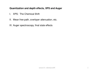
Quantization and depth effects, XPS and Auger • XPS: The Chemical Shift • Mean free path, overlayer attenuation, etc. • Auger spectroscopy, final state effects Lecture 5—chemical shift
The XPS Chemical Shift: Shifts in Core level Binding Energies with Chemical State ΔEChemical Shift In part fromC. Smart, et al., Univ. Hong Kong and UWO
The binding energy is defined as: Eb = hv –Ek –Φ Where hv= photon energy Ek = kinetic energy of the photoelectron Φ = work function of the spectrometer Specifically, the CHEMICAL SHIFT is ΔEb That is the change in Eb relative to some chemical standard Binding energies and particle size
Chemical Shift in Au compounds vs. bulk elemental gold PHI handbook Binding energies and particle size
e- hv Ekin Ekin Evacuum Φspectrometer Evacuum EF EB Because the electron emitted from the solid has to impact on the analyzer/dectector to be counted, the relationship Ekin and EB has to include the work function term of the detector (typically, 4-5 eV): Ekin = hv-EB – Φspectrometer We only need the work function term for the spectrometer, not the sample, because (for a conducting sample) the two Fermi levels are coupled. Obviously, electrically insulating samples present problems (Charging)
e- hv Ekin Ekin Evacuum Φspectrometer Evacuum EF • Changes in EB result from : • Changes in oxidation state of the atom (initial state effect) • Changes in response of the system to the core hole final state: EB mainly sometimes ΔEB = ΔE(in.state) – ΔR + other effects (e.g., band bending) where ΔR = changes in the relaxation response of the system to the final state core hole (see M.K. Bahl, et al., Phys. Rev. B 21 (1980) 1344
ΔEb = kΔqi + ΔVij Vij often similar in different atoms of same material, so Δvij is typically negligible
Initial state term, often similar for diff. atoms in same molecule ΔEb = kΔqi + ΔVij In principle, can be obtained from ground state Mulliken Charge Density calculations Valence charge is removed or added to an atom by interaction with surrounding atoms. Binding energies and particle size
Chemical shift is dominated by changes in ground state valence charge density: • Changes in valence charge density dominated by nearest-neighbor interactions • Qualitative interpretation on basis of differences in ground state electronegativities Binding energies and particle size
e- O withdraws valence charge from C: C(1s) shifts to higher BE relative to elemental C (diamond) at 285.0 eV O C C C C EN = 3.5 EN = 2.5 Elemental C: binding energy = 285.0 eV Ti e- Ti donates charge to C, binding energy shifts to smaller values relative to 285 eV EN = 1.5 Binding energies and particle size
Thus, a higher oxidation state (usually) yields a higher binding energy!
Electron withdrawing groups shift core levels to higher binding energy Binding energies and particle size
Binding energy shifts can be used to follow the course of surface reactions for complex materials: e.g., atomic O /(Pt)NiSi (e.g., Manandhar, et al., Appl. Surf. Sci. 254(2008) 7486 Vacuum Atomic O = Ni = Si Bulk NiSi (Schematic, not real structure) Binding energies and particle size
Pauling Electronegativities, Ground State Si = 1.8 O = 3.5 Ni = 1.8 Ni-O or Si-O formation shift of Ni or Si to higher BE Question: Ni-Si Ni-Ni. Which way should BE move (think). Binding energies and particle size
XPS binding energy shifts for Pt-doped NiSi as a function of exposure to atomic O at room temp. (Manadhar, et al., Appl. Surf. Sci. 254 (2008) 7486 SiO2 Si SiO2 peak appears (shift to higher BE) Ni (2p) shifts to lower BE. Why? Exposure to atomic O
O + O2 Si SiO2 (A) Preferential Si oxidation, Si flux creates metal-rich substrates PtSi Pt1+ySi Si transport and oxidation NiSi Ni1+x Si O + O2 Pt silicate formation (B) Si transport kinetically inhibited, metal oxidation Pt1+y Si Ni1+xSi
How do we estimate q, Δq? This is usually done with Mulliken atomic charge densities, originally obtained by LCAO methods: ΨMO = caΦa + cbΦb Φa(b) atomic orbital on atom a (b) Ψ2 = caca*ΦaΦa* + [cross terms] + cbcb*ΦbΦb* Atomic charge on atom a Atomic charge on atom b Overlap charge
Different Boron Environments in orthocarborane derived films (B10C2HX and B10C2HX:Y) B-B-H C2-B-H RC-B C-B-H Rc=Ring carbon
C2-B B-B-H C2-B-H CB-B C-B-H B2-B Figure 3
Chemical Shifts: Final Note • Calculating ground state atomic charge populations with DFT: • Minimal basis sets give best results (LCAO-MO) • Such basis sets are not best for lowest energy/geometric optimization Binding energies and particle size
Attenuation: hv I = I0 Clean surface of a film or single crystal e- hv I = I0exp(-d/λ) d • Issues: • Average coverage • Calculating λ • Relative vs. Absolute intensities film or single crystal with overlayer of thickness d Binding energies and particle size
Bilayer Surface coverage = Θ2 d = d2 Bare surface Coverage = 1-(Θ1+Θ2) Monolayer Surface coverage = Θ1 d = d1 We can only measure a total intensity from a macroscopic area of the surface: I = [1-(Θ1+Θ2)] I0 + Θ1I0 exp[-d1/λ] + Θ2 1I0 exp[-d2/λ] = I0exp[-dave/λ] we can only determine average coverage with XPS! Binding energies and particle size
Consider 2 cases: • dave < 1 ML (0<Θ<1) • dave> 1 ML (Θ> 1) • We need to look at the RATIO of Isubstrate (IB) and Ioverlayer (IA) • Why? Absolute intensity of IB can be impacted by: • Small changes in sample position • Changes in x-ray flux • IB/IA will remain constant Binding energies and particle size
Calculation of the overlayer coverage First, we need to calculate the IMFP of the electrons of the substrate through the overlayer and the IMFP of the electrons in the overlayer. The formula to calculate the IMFP is (NIST): IMFP=E/Ep2([βln(γE)-(C/E)+(D/E2]) Binding energies and particle size
Terms used in the excel sheet (example Carbon through MgO) After you insert all the four columns, the IMFP is calculated on its own.
=D6*EXP(-A6/26.36) =E6*(1-EXP(-A6/33.17)) =Area under the curve1915/0.25 =Area under the curve 54544/0.66 Binding energies and particle size
Take-off angle variations in XPS: Definition Take off angle (θ) is the angle between the surface normal and the axis of the analyzer. (Some people use 90-θ) Surface normal θ θ = 0 normal emission θ=89 grazing emission
Take-off angle variations in XPS: Intensity vs. θ Intensity of a photoemission peak goes as I ~ I cosθ Therefore, intensities of adsorbates and other species are NOT enhanced at grazing emission (large θ)!
Take-off angle variations in XPS: Sampling Depth (d) normal emission (θ = 0) d ~ λ (inelastic mean free path) λ λ θ increased take-off angle: d~ λcosθ (reduced sampling depth) λcosθ
d~ λ cosθ: Effective sampling depth (d) decreases as θ increases Relative intensities of surface species enhanced relative to those of subsurface: Si SiO2 SiO2 SiO2 λ Si Si SiO2 Si λcosθ
In Dragon and other systems: Arrangement of sample holder may cause increased signal from Ta or other extraneous materials. These should be monitored. However, enhancement of SiO2 relative to Si will remain the same. SiO2 Si Ta sample holders
Multiplet Splitting: • Valence electrons give rise to different spin states (crystal field, etc. Cu 2p 3/2 vs. ½ states • Formation of a core hole shell yields an unpaired electron left in the shell • Coupling between the core electron spin and valence spins gives rise to final states with different total angular momentum. Binding energies and particle size
Multiplet splitting in Cu 2p3/2 2p1/2 Binding energies and particle size
Auger Spectroscopy: Final State Effects XPS initial State XPS Final State hv or e- Auger Final State Auger Initial State Binding energies and particle size
Kinetic Energy of Auger Electron: This transition is denoted as (KLL) e- detector e- Initial state Final State L2,3 (2p) L2,3 (2p) L1 (2s) L1 (2s) K (1s) K (1s) KEAuger = EK - EL1 – EL2,3 - Ueff ~ EK – EL-EL - Ueff Note: Auger transitions are broad, and small changes in BE (EL1 vs. EL2,3 ) sometimes don’t matter that much (sloppy notation) What is Ueff? Binding energies and particle size
L2,3 (2p) L1 (2s) Ueff is the coulombic interaction of the final state holes, as screened by the final state response of the system: e.g., Jennison, Kelber and Rye “Auger Final States in Covalent Systems”, Phys. Rev. B. 25 (1982) 1384 K (1s) Binding energies and particle size
For a typical metal, the final state holes are often delocalized (completely screened), and Ueff ~ 0 eV. However, for adsorbed molecules, or nanoparticles, the holes are constrained in proximity to each other. Ueff can be large, as large as 10 eV or more. Nanoparticle, Ueff ~ 1/R Agglomeration, should see shift in Auger peak as Ueff decreases R Heat in UHV Binding energies and particle size
KE(LVV) = EL –EV – EV – Ueff as particle size increases, Ueff decreases Note shift in Cu(LVV) Auger as nanoparticles on surface agglomerate J. Tong, et al. Appl. Surf. Sci. 187 (2002) 253 Cu/Si:O:C:H Binding energies and particle size
Similar effects in Auger KE are seen for agglomeration during Cu deposition at room temp. (Tong et al.) Cu(LVV) shift with increasing Cu coverage Note corresponding change in Cu(2p3/2) binding energy. Binding energies and particle size
Auger in derivative vs. integral mode When doing XPS, x-ray excited Auger spectra are acquired along with photoemission lines Binding energies and particle size
Auger spectra, though broad, can give information on the chemical state (esp. if the XPS BE shift is small as in Cu(0) vs. Cu(I) Above spectra are presented in the N(E) vs. E mode—or “integral mode” Binding energies and particle size
However, in some cases Auger spectroscopy is used simply to monitor surface cleanliness, elemental composition, etc. This often involves using electron stimulated Auger (no photoemission lines). • Auger spectra are typically broad, and on a rising background. Presenting spectra in the differential mode (dN(E)/dE) eliminates the background. • Peak-to-peak height (rather than peak area) is proportional to total signal intensity, and the background issue is eliminated. Except in certain cases, however, (e.g., C(KVV)) most chemical bonding info is lost. Binding energies and particle size
Auger (derivative mode) of graphene growth on Co3O4(111)/Co(0001) (Zhou, et al., JPCM 24 (2012) 072201 Homework: explain the data on the right. Binding energies and particle size
N(E) KE Peak-to-peak height Binding energies and particle size