Data Compression by Quantization
Data Compression by Quantization. Edward J. Wegman Center for Computational Statistics George Mason University. Outline. Acknowledgements Complexity Sampling Versus Binning Some Quantization Theory Recommendations for Quantization. Acknowledgements.

Data Compression by Quantization
E N D
Presentation Transcript
Data Compression by Quantization Edward J. Wegman Center for Computational Statistics George Mason University
Outline • Acknowledgements • Complexity • Sampling Versus Binning • Some Quantization Theory • Recommendations for Quantization
Acknowledgements • This is joint work with Nkem-Amin (Martin) Khumbah • This work was funded by the Army Research Office
Complexity Descriptor Data Set Size in Bytes Storage Mode Tiny 102 Piece of Paper Small 104 A Few Pieces of Paper Medium 106 A Floppy Disk Large 108 Hard Disk Huge 1010 Multiple Hard Disks e.g. RAID Storage Massive 1012 Robotic Magnetic Tape Storage Silos Super Massive 1015 Distributed Archives The Huber/Wegman Taxonomy of Data Set Sizes
Complexity O(r) Plot a scatterplot O(n) Calculate means, variances, kernel density estimates O(n log(n)) Calculate fast Fourier transforms O(nc) Calculate singular value decomposition of an rc matrix; solve a multiple linear regression O(n2) Solve most clustering algorithms. O(an) Detect Multivariate Outliers Algorithmic Complexity
Motivation • Massive data sets can make many algorithms computationally infeasible, e.g. O(n2) and higher • Must reduce effective number of cases • Reduce computational complexity • Reduce data transfer requirements • Enhance visualization capabilities
Data Sampling • Database Sampling • Exhaustive search may not be practically feasible because of their size • The KDD systems must be able to assist in the selection of appropriate parts if the databases to be examined • For sampling to work, the data must satisfy certain conditions (not ordered, no systematic biases) • Sampling can be very expensive operation especially when the sample is taken from data stored in a DBMS. Sampling 5% of the database can be more expensive that a sequential full scan of the data.
Data Compression • Squishing, Squashing, Thinning, Binning • Squishing = # cases reduced • Sampling = Thinning • Quantization = Binning • Squashing = # dimensions (variables) reduced • Depending on goal, one of sampling or quantization may be preferable
Data Quantization Thinning vs Binning • People’s first thoughts about Massive Data usually is statistical subsampling • Quantization is engineering’s success story • Binning is statistician’s quantization
Data Quantization • Images are quantized in 8 to 24 bits, i.e. 256 to 16 million levels. • Signals (audio on CDs) are quantized in 16 bits, i.e. 65,536 levels • Ask a statistician how many bins to use, likely response is a few hundred, ask a CS data miner, likely response is 3 • For a terabyte data set, 106 bins
Data Quantization • Binning, but at microresolution • Conventions • d = dimension • k = # of bins • n = sample size • Typically k << n
Data Quantization • Choose E[W|Q = yj] = mean of observations in jth bin = yj • In other words, E[W|Q] = Q • The quantizer is self-consistent
Data Quantization • E[W] = E[Q] • If is a linear unbiased estimator, then so is E[|Q] • If h is a convex function, then E[h(Q)] E[h(W)]. • In particular, E[Q2] E[W2] and var (Q) var (W). • E[Q(Q-W)] = 0 • cov (W-Q) = cov (W) - cov (Q) • E[W-P]2 E[W-Q]2 where P is any other quantizer.
Distortion due to Quantization • Distortion is the error due to quantization. • In simple terms, E[W-Q]2. • Distortion is minimized when the quantization regions, Sj, are most like a (hyper-) sphere.
Geometry-based Quantization • Need space-filling tessellations • Need congruent tiles • Need as spherical as possible
Geometry-based Quantization • In one dimension • Only polytope is a straight line segment (also bounded by a one-dimensional sphere). • In two dimensions • Only polytopes are equilateral triangles, squares and hexagons
Geometry-based Quantization • In 3 dimensions • Tetrahedrons (3-simplex), cube, hexagonal prism, rhombic dodecahedron, truncated octahedron. • In 4 dimensions • 4 simplex, hypercube, 24 cell Truncated octahedron tessellation
Geometry-based Quantization Tetrahedron* .1040042… Cube* .0833333… Octahedron .0825482… Hexagonal Prism* .0812227… Rhombic Dodecahedron* .0787451… Truncated Octahedron* .0785433… Dodecahedron .0781285… Icosahedron .0778185… Sphere .0769670 Dimensionless Second Moment for 3-D Polytopes
Geometry-based Quantization Tetrahedron Cube Octahedron Truncated Octahedron Dodecahedron Icosahedron
Geometry-based Quantization Rhombic Dodecahedron http://www.jcrystal.com/steffenweber/POLYHEDRA/p_07.html
Geometry-based Quantization 24 Cell with Cuboctahedron Envelope Hexagonal Prism
Geometry-based Quantization • Using 106 bins is computationally and visually feasible. • Fast binning, for data in the range [a,b], and for k bins j = fixed[k*(xi-a)/(b-a)] gives the index of the bin for xi in one dimension. • Computational complexity is 4n+1=O(n). • Memory requirements drop to 3k- location of bin + # items in bin + representor of bin, I.e. storage complexity is 3k.
Geometry-based Quantization • In two dimensions • Each hexagon is indexed by 3 parameters. • Computational complexity is 3 times 1-D complexity, • I.e. 12n+3=O(n). • Complexity for squares is 2 times 1-D complexity. • Ratio is 3/2. • Storage complexity is still 3k.
Geometry-based Quantization • In 3 dimensions • For truncated octahedron, there are 3 pairs of square sides and 4 pairs of hexagonal sides. • Computational complexity is 28n+7 = O(n). • Computational complexity for a cube is 12n+3. • Ratio is 7/3. • Storage complexity is still 3k.
Quantization Strategies • Optimally for purposes of minimizing distortion, use roundest polytope in d-dimensions. • Complexity is always O(n). • Storage complexity is 3k. • # tiles grows exponentially with dimension, so-called curse of dimensionality. • Higher dimensional geometry is poorly known. • Computational complexity grows faster than hypercube.
Quantization Strategies • For purposes of simplicity, always use hypercube or d-dimensional simplices • Computational complexity is always O(n). • Methods for data adaptive tiling are available • Storage complexity is 3k. • # tiles grows exponentially with dimension. • Both polytopes depart spherical shape rapidly as d increases. • Hypercube approach is known as datacube in computer science literature and is closely related to multivariate histograms in statistical literature.
Quantization Strategies • Conclusions on Geometric Quantization • Geometric approach good to 4 or 5 dimensions. • Adaptive tilings may improve rate at which # tiles grows, but probably destroy spherical structure. • Good for large n, but weaker for large d.
Quantization Strategies • Alternate Strategy • Form bins via clustering • Known in the electrical engineering literature as vector quantization. • Distance based clustering is O(n2) which implies poor performance for large n. • Not terribly dependent on dimension, d. • Clusters may be very out of round, not even convex. • Conclusion • Cluster approach may work for large d, but fails for large n. • Not particularly applicable to “massive” data mining.
Quantization Strategies • Third strategy • Density-based clustering • Density estimation with kernel estimators is O(n). • Uses modes m to form clusters • Put xi in cluster if it is closest to mode m. • This procedure is distance based, but with complexity O(kn) not O(n2). • Normal mixture densities may be an alternative approach. • Roundness may be a problem. • But quantization based on density-based clustering offers promise for both large d and large n.
Data Quantization • Binning does not lose fine structure in tails as sampling might. • Roundoff analysis applies. • With scale of binning, discretization not likely to be much less accurate than accuracy of recorded data. • Discretization - finite number of bins implies discrete variables more compatible with categorical data.
Data Quantization • Analysis on a finite subset of the integers has theoretical advantages • Analysis is less delicate • different forms of convergence are equivalent • Analysis is often more natural since data is already quantized or categorical • Graphical analysis of numerical data is not much changed since 106 pixels is at limit of HVS