Survey of Quantization
1.17k likes | 3.13k Vues
Survey of Quantization. Itai Katsir. References. [1] Gray, R.M.; Neuhoff, D.L., “ Quantization” , IEEE Transactions on Information Theory, Volume 44, Issue 6, Oct. 1998 Page(s):2325 – 2383.

Survey of Quantization
E N D
Presentation Transcript
Survey of Quantization Itai Katsir
References • [1] Gray, R.M.; Neuhoff, D.L., “Quantization”, IEEE Transactions on Information Theory, Volume 44, Issue 6, Oct. 1998 Page(s):2325 – 2383. • [2] Goyal, V.K., “Theoretical foundations of transform coding”, IEEE Signal Processing Magazine, Volume 18, Issue 5, Sep 2001 Page(s):9 – 21. • [3] N.S. Jayant and P. Noll, Digital Coding of Waveforms, Prentice-Hall, 1984. • [4] A. Gersho and R.M. Gray, Vector Quantization and Signal Compression, Kluwer, 1991. • [5] Y. Linde, A. Buzo and R. Gray, “An Algorithm for Vector Quantizer Design”, IEEE Trans. Commun. Vol. COM-28, No. 1, Jan. 1980, pp. 84-95.
Agenda • Introduction. • Uniform Quantization. • Non-Uniform Quantization. • Adaptive Quantization. • Predictive Quantization. • Vector Quantization. • Applications. • Discussion.
Agenda • Introduction. • Uniform Quantization. • Non-Uniform Quantization. • Adaptive Quantization. • Predictive Quantization. • Vector Quantization. • Applications. • Discussion.
Introduction • Most signals are analog in nature. • Most systems in nature operate in continuous time. • Computer handles discrete data. • To store, transmit or manipulate signals, they first must be digitized. • Two aspects: • Temporal/spatial sampling. • Amplitude and coefficient quantization.
Sampling Amplitude-continues, Time-continues Amplitude-continues, Time-discrete 11 Quantizing 10 01 00 Amplitude- discrete, Time-discrete Introduction Sampling and quantization of an analog signal.
IntroductionImage Example: • Sampling • Sample the value of the image at the nodes of a regular grid on the image plane. • A pixel (picture element) at (i, j) is the image intensity value at grid point indexed by the integer coordinate (i, j).
256x256 64x64 16x16 Introduction Examples of Sampling
IntroductionImage Example: Quantization Is a process of transforming a real valued sampled image to one taking only a finite number of distinct values. Each sampled value in a 256-level grayscale image is represented by 8 bits. 255 (white) 0 (black)
8 bits / pixel 4 bits / pixel 2 bits / pixel Introduction Examples of Quantization
Introduction Quantization in signal processing systems: A-to-D convert Transform coding (encoder)
Introduction The problems: Quantization is an irreversible process. Quantization is a source of information loss. Quantization is a critical stage in signals compression, with impact on: the distortion of reconstructed signals. the bit rate of the encoder. The goal – optimal or high quality quantizer: Smallest average distortion (marked D). Lowest rate (marked R).
Agenda • Introduction. • Uniform Quantization. • Non-Uniform Quantization. • Adaptive Quantization. • Predictive Quantization. • Vector Quantization. • Applications. • Discussion.
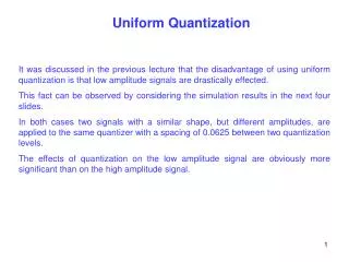
Uniform Quantization All quantization decision regions are of equal size Except first and last regions if samples are not finite valued. The quantizing levels are the midpoint of the decision levels. With N quantization regions,use B=log2(N) bits to represent each quantized value.
Uniform Quantization Quantizer distortion: Quantizer rate:
Uniform QuantizationQuantization Error (Noise) • Quantization error (rounding): • Error bounds: Overload quantization noise Granular quantization noise
Uniform QuantizationNoise Analysis Assumption: The noise signal and the input signal are uncorrelated. Under certain assumptions, notably smooth input probability density functions and high rate quantizers, the noise signal acts like a white noise sequence. Few samples clipped. The amplitudes of noise samples are uniformly distributed across the range: resulting in average power:
Uniform QuantizationNoise Analysis Signal-to-quantization-noise ratio of B bits uniform quantizer: Signal-to-quantization-noise ratio (in dB): We get
Uniform QuantizationOptimal Quantizer For optimal quantization, minimize with respect to : For a uniform PDF:(1bit quantizer) In general, the optimal step size is proportional to the standard deviation for a given pdf, , shown in the next table:
Agenda • Introduction. • Uniform Quantization. • Non-Uniform Quantization. • Adaptive Quantization. • Predictive Quantization. • Vector Quantization. • Applications. • Discussion.
Non-Uniform Quantization Signals PDF has tails (Gaussian, Laplacian, etc.). Smaller signal input magnitude (more likely input) should be more accurate quantized. Larger signal input magnitude (less likely input) should be coarsely quantized. Gives lower mean square quantization noise with the same bit rate.
Non-Uniform Quantization Quantizer distortion as in uniform quantizer: Both the decision level and the quantizing level can vary. Optimal condition for minimum distortion: Impossible to solve analytically.
Non-Uniform QuantizationLloyd-Max Algorithm Lloyd-Max: iterative numerical algorithm for optimal quantizer. Set initial values to . set k=1 Calculate Calculate If k=N go to (5) else k=k+1 and go to (2).
Non-Uniform QuantizationLloyd-Max Algorithm Calculateif stop else go to (6) Calculate set k=1 and go to (2).
Non-Uniform QuantizationLloyd-Max Algorithm Quantization decision regions are densely located in the center region and coarsely elsewhere. The decision level are halfway between neighboring quantizing levels (nearest neighbor). The quantizing levels are the centroid of the PDF over the appropriate interval. Example of optimal non-uniform quantizer decision points for Laplacian PDF:
Non-Uniform QuantizationOptimal Quantizer Example of uniform and non-uniform optimal Laplacian distributor quantizer:
Non-Uniform QuantizationCompanding Non-uniform quantizer designed from a uniform quantizer and a non-linear component. Robustness to PDF changes,especially signal magnitudechanges. Used widely for PCM telephony ( ).
Agenda • Introduction. • Uniform Quantization. • Non-Uniform Quantization. • Adaptive Quantization. • Predictive Quantization. • Vector Quantization. • Applications. • Discussion.
Adaptive Quantization • Uniform quantization: fixed quantization region • Non-uniform quantization: variable quantization region which are fixed over time. • Adaptive quantization: • The quantization region is varied over time. • The quantizer is adapted to changing input signal statistics. • Achieves lower distortion - better performance. • Cost in extra processing delay and an extra storage requirement. • General quantization region calculation:
Adaptive Quantization • Forward adaptive quantization • The encoder estimate the best quantization regions from input sequence. This estimation is transmitted to the decoder instantaneous or over a block of samples. • Add side information of statistical parameters.
Adaptive Quantization Forward adaptive quantization • The selection of block size is a critical issue. • If the size is small, the adaptation to the local statistics will be effective, but the side information needs to be sent frequently. (more bits used for sending the side information). • If the size is large, the bits used for side information decrease. The adaptation becomes less sensitive to changing statistics, and both processing delay and storage required increase. • In practice, a proper compromise between quantity of side information and effectiveness of adaptation produces a good selection of the block size.
Adaptive Quantization • Backward adaptive quantization • The encoder and decoder execute the same algorithm for estimating the quantization regions. • The estimation is based on quantized samples.
Adaptive Quantization Backward adaptive quantization • There is no need to send side information. • The sensitivity of adaptation to the changing statistics will be degraded because of using the quantize signal instead of the original input. That is, the quantization noise is involved in the statistical analysis.
Adaptive Quantization • Adaptive quantization with one word memory (Jayant quantizer) • Uses one input sample in forward adaptation or one output sample in backward adaptation. • Input/output sample that falls into quantization region i at time (n)changes the region size bymi at time (n+1).
Agenda • Introduction. • Uniform Quantization. • Non-Uniform Quantization. • Adaptive Quantization. • Predictive Quantization. • Vector Quantization. • Applications. • Discussion.
Predictive Quantization • instead of encoding a signal directly, the differential coding technique encodes the difference between the signal itself and its prediction. Therefore it is also known as predictive coding.
Predictive Quantization • The error prediction signalhas much smaller variancecompared to the originalinput signal variance. • Allow smaller quantizationregion of the quantizer. • Example of image histogramcompared to the histogram of the difference image:
Agenda • Introduction. • Uniform Quantization. • Non-Uniform Quantization. • Adaptive Quantization. • Predictive Quantization. • Vector Quantization. • Applications. • Discussion.
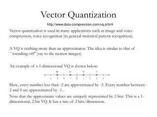
Vector Quantization • maps k-dimensional vectors in the vector space into a finite set of vectors . • Each vector is called a code-vector or a codeword. and the set of all the codewords, , is called a codebook. • The codebook vectors are selected through a clustering or training process, involving representative source training data.
Vector Quantization • Major problem of VQ is its very high computational complexity. Resolves from the search algorithm of the correct codeword for received input vector. • Quantizer rate:
Vector Quantization • Associated with each codeword, , is a nearest neighbor region called Voronoi region, and it is defined by: • The set of Voronoi regions partition the entire space .
Vector QuantizationExample – Voroni Region • Example of two dimensional (k=2) Voroni region of non-uniform source PDF: • Input vectors aremarked with an x,codewords are markedwith red circles, and the Voronoi regions are separated with boundary lines.
Vector QuantizationSchema: • Allow very low rate encoding. • Very high computational complexity. • The higher the value N the better quality, but lower compression ratio.
Vector QuantizationCodebook Design Problem • Given a training sequence consisting of M>10N source vectors (M is sufficiently large to capture all statistics properties of source) of k dimension: • Given the number of codevectors: • Find a codebook , Find a partition • which result in the smallest average distortion:
Vector QuantizationCodebook Design • General Lloyd (GL) algorithm: • Determine the number of codewords, N, or the size of the codebook. • Select N codewords at random, and let that be the initial codebook. The initial codewords can be randomly chosen from the set of input vectors. • Using the Euclidean distance measure, D, clusterize the vectors around each codeword. This is done by taking each input vector and finding the Euclidean distance between it and each codeword. The input vector belongs to the cluster of the codeword that yields the minimum distance.
Vector QuantizationCodebook Design • GL algorithm (cont.): • Compute the new set of codewords. This is done by obtaining the average (the centroid) of each cluster. Add the component of each vector and divide by the number of vectors in the cluster. where i is the cluster number, m is the number of vectors in the cluster. • Repeat steps (3) and (4) until the average distortion is small enough: • Problem – the codewords may fall into local minimum, depends on the initial selected codebook. • One solution – the LBG algorithm which uses splitting method.
Vector QuantizationCodebook Design • LBG algorithm: • Set N*=1 and calculate initial codebook:and calculate initial Euclidean distance D* • Splitting: For i=1,2,…, N* setSet N*=2N*. • Iteration: Use GL algorithm steps (3)-(5) to find optimal codewords. • Repeat (3) and (4) until the desired number of codewords, N, is obtained.
Vector QuantizationCodebook Design • LBG algorithm: • Animation
Vector QuantizationCodebook Design • Example of image VQ codebook (N=256):