Download
1 / 32
320 likes | 342 Vues
Explore the process of injecting signals into LIGO for testing purposes, validating efficiency calculations, and signal detection accuracy. The project aims to understand signal dependencies and optimize detection confidence.

E N D
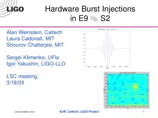
Hardware Burst Injections in E9 S2 Alan Weinstein, Caltech Laura Cadonati, MIT Shourov Chatterjee, MIT Sergei Klimenko, UFla Igor Yakushin, LIGO-LLO LSC meeting, 3/18/03 AJW, Caltech, LIGO Project
Goals of the Burst Injections • test our understanding of the entire signal chain from • GDS excitation point • displacements of test masses • data logged in LSC-AS_Q and related DM and common mode channels • entire burst search analysis chain. • In particular, we need a quantitative comparison between signals injected into the IFO and signals injected into the datastream in software (in LDAS), to validate the efficiency calculation. • Verify that we detect HW injected signals with SNR as expected • Detection confidence • Test our understanding of the dependence on source direction and polarization. AJW, Caltech, LIGO Project
Injecting signals The multiawgstream and SIStr facilities developed by I. Leonor, P. Shawhan, D. Sigg are used to inject series of signals into the LSC-ETMX_EXC, and LSC-ETMY_EXC, or DARM_CTRL_EXC channels of the three interferometers. The injections during S1, E9 and S2 were/are coordinated by M. Landry, P. Shawhan, S. Marka Many thanks to all the developers for this immensely important and useful facility! AJW, Caltech, LIGO Project
Original (ambitious) program:Burst_z and Burst_ang Burst_z scan, into DARM or ETMX-ETMY: • inject sine-Gaussians into all 6 end test masses, with durations of ~ 1 second, spaced 40 seconds apart. • Scan 8 logarithmically-spaced central frequencies from 100 - 2000 Hz. • Scan ~6 amplitudes from 1 to 100 times the nominal calibrated strain sensitivity at that central frequency. • These 48 bursts should thus take 32 minutes. Burst_ang scan, exciting both DARM and CARM, with IFO-IFO delays: • Choose one central frequency and relatively large amplitude, and scan over 100 source directions and polarizations (5 in cos, 5 in , 4 in ; all with respect to the mean of the LHO/LLO zenith and orientation). This should take 67 minutes. AJW, Caltech, LIGO Project
Frequency f0 (Hz) Duration (msec) 100 90 153 58 235 38 361 25 554 16 850 11 1304 7 2000 4.5 Time from segment start t0 (sec) 20 40 60 80 100 120 140 160 Waveforms, amplitudes • Short, narrow-bandwidth signals (sine-Gaussians) provide the most direct and useful interpretation of IFO and data analysis responses. We envision a "swept-sine calibration" of sine-Gaussians of varying frequency, spanning the LIGO band of interest. • Signal amplitudes should span the range from "barely detectable" to "large, but not so large as to excite a non-linear response". The IFO strain sensitivity varies over the frequency range of interest, so the amplitudes should vary as well. • Signals are injected using the GDS excitation engine, which accepts 16384-Hz time series in units of counts to the coil driver. The frequency dependence of the test mass response must be taken into account. • Each sine-Gaussian has Q ~ 9; total duration ~ Q/f0 AJW, Caltech, LIGO Project
Ad-hoc signals: (Sine)-Gaussians SG 554, Q = 9 These have no astrophysical significance; But are well-defined in terms of waveform, duration, bandwidth, amplitude AJW, Caltech, LIGO Project
Schedule of Signal Injections During the S2 Run Feb 14 2:48 CST, 0:48 PST # Feb 18 23:00 CST, 21:00 PST Feb 23 16:00 CST, 14:00 PST Feb 25 18:00 CST, 16:00 PST * Mar 2 14:00 CST, 12:00 PST Mar 3 12:00 CST, 10:00 PST Mar 7 2:00 CST, 0:00 PST Mar 12 20:00 CST, 18:00 PST Mar 15 24:00 CST, 22:00 PST * Mar 19 23:00 CST, 21:00 PST Mar 23 3:00 CST, 1:00 PST Mar 25 22:00 CST, 20:00 PST Mar 28 20:00 CST, 18:00 PST * Apr 2 10:00 CST, 8:00 PST Apr 5 4:00 CST, 2:00 PST Apr 9 24:00 CST, 22:00 PST * Apr 11 22:00 CDT, 20:00 PDT * inserted during the run to make up for lost opportunities (sometimes the interferometers were just out of lock and injection was pointless or partial) # The injection time was determined just before the injection S, Marka, P. Shawhan, I. Leonor AJW, Caltech, LIGO Project
Actually done and analyzed (so far): • Groups of 8 SG’s, varying amplitudes. • Intra-run injections subject to IFO availability. AJW, Caltech, LIGO Project
Signal amplitudes # Time Cfg Waveform file ETMX ETMY hpeak (strain) 729154547.000000 1 wfsg100Q9.dat 0.0107060 -0.0104160 3.0e-19 729154567.000000 1 wfsg153Q9.dat 0.0312080 -0.0303660 3.7e-19 729154587.000000 1 wfsg235Q9.dat 0.0227440 -0.0221300 1.1e-19 729154607.000000 1 wfsg361Q9.dat 0.0663000 -0.0645080 1.4e-19 729154627.000000 1 wfsg554Q9.dat 0.1932700 -0.1880460 1.7e-19 729154647.000000 1 wfsg850Q9.dat 0.5634020 -0.5481760 2.1e-19 729154667.000000 1 wfsg1304Q9.dat 6.5694940 -6.3919400 1.1e-18 729154687.000000 1 wfsg2000Q9.dat 19.1507320 -18.6331460 1.3e-18 The waveform files have a peak amplitude (at 0.5 secs) of 1. You can read off the ETMx and ETMy signals, peak amplitude in counts. So: |ETMx-ETMy| (in counts) (~1 nm / ct) (DC calibration, approximate, varies from ~0.5-1.0) (0.744/f0)^2 (pendulum response, where f0 is central SG frequency) / 4000 m (or 2000 m for H2) will give you a peak amplitude in strain. AJW, Caltech, LIGO Project
SG injections: frequencies, amplitudes • SG central • frequencies • f0 are color-coded • Closed circles are • detected bursts; • Open circles are • undetected (H1) AJW, Caltech, LIGO Project
Analysis • Data were analyzed through the standard Burst pipeline • Pre-filtering in datacond, including 100 Hz HPF and whitening • For the first few injection runs, HPF 150 Hz and S1 whitening • Then, data from each IFO were passed through tfclusters and slope ETG’s • Each ETG returns triggers with start_time and trigger strength • tfclusters also returns a central frequency • Time resolution: • tfclusters uses time bins of 1/8 second, start_time is quantized in those units (125 msec) • Slope is expected to give < 50 msec resolution AJW, Caltech, LIGO Project
Trigger power (tfclusters)Feb 13 injections Before frequency consistency cut After frequency consistency cut L. Cadonati AJW, Caltech, LIGO Project
TFCLUSTERS central frequency vs injected frequency The red, off diagonal events are the ones rejected by the frequency cut (background noise). The blue, off diagonal events have large bandwidth, covering the injected frequency, thus pass the frequency cut. AJW, Caltech, LIGO Project
Timing accuracy • Injection peaks at 0.5 secs, starts ~10’s of msec before then • Tfclusters (left) is quantized in bins of 1/8 sec. • Slope (right) peak is 10 msec before 0.5 sec. AJW, Caltech, LIGO Project
ETG strength ~ xrms2 • There’s a lot of scatter, but most injections indeed show strength ~ xrms2 • Don’t compare the different colors; they’re different frequencies, and the IFOs have different sensitivities. The black dots are at 100 Hz, and we hpf’ed at 150 Hz! • Still, a lot of signals were not found – under investigation! AJW, Caltech, LIGO Project
H1 – L1 cross-correlation Filtered AS_Q data streams 554 Hz SG at hrms ~ 2e-20 Injected in H1 and L1 simultaneously Correlation coefficient and confidence L. Cadonati AJW, Caltech, LIGO Project
Intra-run injections and stability • A much more limited set of injections are being done throughout S1. • Oops! Used different pre-filtering for the 3/7/03 injections! • Need to run with the new filters on all injections; trying to get the data and filters all available at one ldas… AJW, Caltech, LIGO Project
Comparison with SW injections • Comparison currently only available for latest round of intra-run injections into H1. • Solid points = HW • Open diamonds = SW • Find 45o line connecting points and diamonds of same color (f0)? • That’s qualitative evidence that HW and SW injections with same (nominal) xrms are found by tfclusters with same strength. • Much more work, statistics, etc, required to establish this quantitatively! AJW, Caltech, LIGO Project
Results from WaveBurst • WaveBurst DSO (S. Klimenko, I. Yakushin) cross-correlates data streams from 2 detectors in wavelet basis. • Run on H1 and H2 detectors, using the 23 groups of 8 SG bursts from Feb 13, 2003 • Biorthogonal wavelet of 16th order was used • WaveBurst TF resolution of 1/32 sec x 16 Hz AJW, Caltech, LIGO Project
Central frequency from WaveBurst AJW, Caltech, LIGO Project
WaveBurst power AJW, Caltech, LIGO Project
Central time of WaveBurst cluster AJW, Caltech, LIGO Project
Summary • HW Burst injections, pre-S2 and during S2, are a powerful tool for honing algorithms, building confidence in detection ability, monitoring detection stability, finding problems • Confirms ability to detect bursts at ~ expected level • Comparison of HW and SW injections: qualitatively, in the right ballpark • Failure to detect some signals with tfclusters is under investigation AJW, Caltech, LIGO Project
Signal sent to GDS system The signal that is sent to each of the ETMs by the GDS system is a product of factors: • A waveform with units of strain, sampled at 16384 Hz, is input to the system. • The peak strain amplitude can be scaled to a desired value. • This is multiplied by the arm length (2000 m for H2 and 4000 m for L1), and by “antenna pattern” factors (for the two ETMs in each of the 3 interferometers) corresponding to a particular source direction and polarization. • From the calibration6, we know how many DAC counts, G, correspond to a motion of 1 nm, at frequencies much below the pendulum frequency (fp = 0.74 Hz). G is typically on the order of 1 nm/count. • Since sine-Gaussians are narrow band, with central frequency fc, there is a factor of (fc / fp )2 to account for the pendulum response to force from the GDS-controlled coil actuators. (more complicated filtering would be required for broad-band signals). • Relative delays between the three interferometers are calculated based on the source direction (on the order of msec). AJW, Caltech, LIGO Project
Driver files for injections BURST_Z #T_off filename H2_DELAY M_ETMX M_ETMY L1_DELAY M_ETMX M_ETMY H1_DELAY M_ETMX M_ETMY # (s) (s) (s) (s) 40 wf100.dat 1.0000 0.0544 -0.0536 1.0000 0.0275 -0.0291 1.0000 0.0516 -0.0452 80 wf153.dat 1.0000 0.0640 -0.0630 1.0000 0.0647 -0.0686 1.0000 0.1215 -0.1063 120 wf235.dat 1.0000 0.0753 -0.0742 1.0000 0.0761 -0.0807 1.0000 0.2859 -0.2502 160 wf361.dat 1.0000 0.0354 -0.0349 1.0000 0.0716 -0.0760 1.0000 0.6729 -0.5888 200 wf554.dat 1.0000 0.0417 -0.0411 1.0000 0.0674 -0.0715 1.0000 1.5837 -1.3858 240 wf850.dat 1.0000 0.0981 -0.0967 1.0000 0.1587 -0.1683 1.0000 3.7274 -3.2614 280 wf1304.dat 1.0000 0.2310 -0.2275 1.0000 0.4670 -0.4952 1.0000 17.5450 -15.3519 320 wf2000.dat 1.0000 0.5436 -0.5355 1.0000 1.9783 -2.0979 1.0000 61.9395 -54.1970 360 wf100.dat 1.0000 0.2718 -0.2678 1.0000 0.1374 -0.1457 1.0000 0.2581 -0.2258 400 wf153.dat 1.0000 0.3199 -0.3151 1.0000 0.3233 -0.3429 1.0000 0.6074 -0.5315 … BURST_ANG #T_off filename H2_DELAY M_ETMX M_ETMY L1_DELAY M_ETMX M_ETMY H1_DELAY M_ETMX M_ETMY # (s) (s) (s) (s) 40 wf850.dat 0.0000 1.8795 -1.9080 -0.0000 -3.1329 3.2244 0.0000 71.3846 -64.3627 80 wf850.dat -0.0038 0.7602 -1.8054 0.0038 -2.3396 0.2829 -0.0038 28.8713 -60.9012 120 wf850.dat -0.0038 0.4389 -1.2321 0.0038 -0.9553 0.1659 -0.0038 16.6688 -41.5612 160 wf850.dat -0.0038 0.0000 -0.3286 0.0038 0.6849 0.0045 -0.0038 0.0000 -11.0849 200 wf850.dat -0.0043 1.0065 -1.2559 0.0043 -0.9788 0.6367 -0.0043 38.2277 -42.3656 240 wf850.dat -0.0043 0.7087 -0.4360 0.0043 0.4348 0.7272 -0.0043 26.9171 -14.7080 280 wf850.dat -0.0043 0.2210 0.5007 0.0043 1.7320 0.6229 -0.0043 8.3941 16.8906 320 wf850.dat -0.0043 -0.3259 1.3033 0.0043 2.5650 0.3516 -0.0043 -12.3781 43.9634 360 wf850.dat -0.0042 1.3805 -0.6045 0.0042 -0.0302 1.5366 -0.0042 52.4316 -20.3904 AJW, Caltech, LIGO Project
First look at 8/17/02 injections into L1:LSC-DARM_CTRL_EXC • Beginning with 360 seconds of injections (one every 40 seconds) with scale factors 7.5 and 30 • Command: darm_z_burst 713668660 1 • Can we see the signals in the time series? • Can we see the signals in spectrograms? • Can the burst search DSOs see the signals? • Do we quantitatively understand the amplitude of the signals? Do they compare well with software injections into the data stream in LDAS? AJW, Caltech, LIGO Project
Can we see the signals in the time series? • Surely not, given the very large low frequency noise. • But we can zoom in, A LOT. (eg, zoom in on 235 Hz SG at 121 seconds after start). • Or, we can HP filter the data. (eg, 10th order Butterworth at 120 Hz) 235 Hz wiggle here! AJW, Caltech, LIGO Project
Can we see the signals in the spectrogram? • Surely not, unless you really zoom in. • But this shows that it’s a pretty quiet stretch of data. AJW, Caltech, LIGO Project
Zoom in on the spectrogram 100 Hz at 41 sec 153 Hz at 81 sec 235 Hz at 121 sec 361 Hz at 161 sec 554 Hz at 201 sec 2000 Hz at 321 sec AJW, Caltech, LIGO Project
Can we see it in tfclusters? • tfclusters (J. Sylvestre) is one of our well-tested burst search algorithms, running in LDAS as a wrapperAPI DSO • It calculates excess power in pixels in the t-f plane, then looks for clusters of such pixels. • It generates a list of triggers, with start_time, burst power, central frequency, bandwidth, duration. AJW, Caltech, LIGO Project
100 153 235 361 554 850 1304 2000 tfclusters triggers • Triggers in time with injected bursts are indicated in red • For scale factor 7.5, we find bursts above 150 Hz with large SNR • Trigger “power” scales like (30/7.5)2 as expected scale factor 30 scale factor 7.5 AJW, Caltech, LIGO Project
Amplitude • The real point of all this is to “cross-calibrate” hardware vs software injections, testing our understanding of all the gain factors. • First check: injections into LLO with scale factors differing by factor 4, show up in tfclusters with “power” differing by ~ 42. OK! • This work is in progress. AJW, Caltech, LIGO Project