Graphs
Explore the fundamentals of graph theory, key definitions, properties, operations, and applications. Understand graphs, tree structures, traversals (DFS, BFS), spanning trees, connected components, and more. Ideal for students and enthusiasts.


Graphs
E N D
Presentation Transcript
Graphs 2014, Fall Pusan National University Ki-Joune Li
b c a a e d d c b e Graph • Definition • G = (V,E ) where V : a set of vertices and E = { <u,v> | u,v V } : a set of edges • Some Properties • Equivalence of Graphs • Tree • a Graph • Minimal Graph
Some Terms • Directed Graph • G is a directed graph iff <u,v> <v,u > for uv V • Otherwise G is an undirected graph • Complete Graph • Suppose nv= number(V ) • Undirected graph G is a complete graph if ne= nv (nv - 1) / 2, where neis the number of edges • Adjacency • For a graph G=(V,E ) u is adjacent to v iff e = <u,v> E , where u,v V • If G is undirected, v is adjacent to uotherwise v is adjacent from u
Some Terms • Subgraph • G’ is a subgraph of a graph G iffV (G’ ) V (G ) and E (G’ ) E (G ) • Path from u to v • A sequence of vertices u=v0, v1, v2, … vn=v V , such that<vi ,vi +1> E for every vi • Cycle iff u = v • Connected • Two vertices u and v are connected iff a path from u to v • Graph G is connected iff for every pair u and v there is a path from u to v • Connected Components • A connected subgraph of G
Some Terms • Connected • An directed graph G is strongly connected iffiff for every pair u and v there is a path from u to v and path from v to u • DAG: directed acyclic graph (DAG) • In-degree and Out-Degree • In-degree of v : number of edges coming to v • Out-degree of v : number of edges going from v
0 1 2 3 Representation of Graphs: Matrix • Adjacency Matrix • A[i, j ] = 1, if there is an edge <vi ,vj >A[i, j ] = 0, otherwise • Example • Undirected Graph: Symmetric Matrix • Space complexity: O (nv2 ) bits • In-degree (out-degree) of a node
0 0 1 2 3 1 1 2 2 2 3 3 3 Representation of Graphs: List • Adjacency List • Each node has a list of adjacent nodes • Space Complexity: O (nv + ne ) • Inverse Adjacent List 0 1 0 2 0 1 3 0 2
0 1.5 1 2.3 1.2 1.0 2 3 1.9 0 1 1.5 2 2.3 3 1.2 1 2 1.0 2 3 1.9 3 Weighted Graph: Network • For each edge <vi ,vj >, a weight is given • Example: Road Network • Adjacency Matrix • A[i, j ] = wij, if there is an edge <vi ,vj > and wijis the weight A[i, j ] = , otherwise • Adjacency List
0 1 4 2 3 5 6 7 Graph: Basic Operations • Traversal • Depth First Search (DFS) • Breadth First Search (BFS) • Used for search • Example • Find Yellow Node from 0
DFS: Depth First Search void Graph::DFS() { visited=new Boolean[n]; for(i=0;i<n;i++)visited[i]=FALSE; DFS(0); delete[] visited; } 0 1 4 2 3 void Graph::DFS(int v) { visited[v]=TRUE; for each u adjacent to v { if(visited[u]==FALSE) DFS(u); } } 5 6 7 Adjacency List: Time Complexity: O(e) Adjacency Matrix: Time Complexity: O(n2)
BFS: Breadth First Search void Graph::BFS() { visited=new Boolean[n]; for(i=0;i<n;i++)visited[i]=FALSE; Queue *queue=new Queue; queue.insert(v); while(queue.empty()!=TRUE) { v=queue.delete() for every w adjacent to v) { if(visited[w]==FALSE) { queue.insert(w); visited[w]=TRUE; } } } delete[] visited; } 0 1 4 2 3 5 6 7 Adjacency List: Time Complexity: O(e) Adjacency Matrix: Time Complexity: O(n2)
Spanning Tree • A subgraph T of G = (V,E ) is a spanning tree of G • iff T is tree and V (T )=V (G ) • Finding Spanning Tree: Traversal • DFS Spanning Tree • BFS Spanning Tree 0 1 4 2 3 5 6 7 0 0 1 1 4 4 2 2 3 3 5 5 6 6 7 7
Articulation Point and Biconnected Components • Articulation Point • A vertex v of a graph G is an articulation point iffthe deletion of v makes G two connected components • Biconnected Graph • Connected Graph without articulation point • Biconnected Components of a graph 0 0 1 1 7 1 4 2 6 7 5 3 4 2 2 6 6 5 3
Finding Articulation Point: DFS Tree • Back Edge and Cross Edge of DFS Spanning Tree • Tree edge: edge of tree • Back edge: edge to an ancestor • Cross edge: neither tree edge nor back edge • No cross edge for DFS spanning tree 2 0 Back edge 1 6 1 7 0 4 4 2 6 3 5 3 5 Back edge 7
Finding Articulation Point • Articulation point • Root is an articulation point if it has at least two children. • u is an articulation point if child of u without back edge to an ancestor of u 2 Back edge 1 6 0 4 3 5 Back edge 7
Finding Articulation Point by DFS Number • DFS number of a vertex: dfn (v ) • The visit number by DFS • Low number: low (v ) • low (v )= min{ dfn (v), min{dfn (x)| (v, x ): back edge }, min{low (x)| x : child of v } } • v is an articulation Point • If v is the root node with at least two children or • If v has a child u such that low (u) dfn (v) • v is the boss of subtree: if v dies, the subtree looses the line 0 0 2 1 1 6 0 5 5 0 4 3 2 2 3 5 0 6 5 4 5 7 7 0
Computation of dfs(v) and low(v) void Graph::DfnLow(x) { num=1; // num: class variable for(i=0;i<n;i++) dfn[i]=low[i]=0; DfnLow(x,-1);//x is the root node } void Graph::DfnLow(int u,v) { dfn[u]=low[u]=num++; for(each vertex w adjacent from u){ if(dfn[w]==0) // unvisited w DfnLow(w,u); low[w]=min(low[u],low[w]); else if(w!=v) low[u]=min(low[u],dfn[w]); //back edge } } Adjacency List: Time Complexity: O(e) Adjacency Matrix: Time Complexity: O(n2)
0 5 1 7 12 3 4 4 2 6 8 2 6 5 3 Minimum Spanning Tree • G is a weighted graph • T is the MST of G iff T is a spanning tree of G and for any other spanning tree of G, C (T ) < C (T’ ) 0 7 5 1 7 10 12 3 4 4 2 6 8 2 6 15 5 3
Finding MST • Greedy Algorithm • Choosing a next branch which looks like better than others. • Not always the optimal solution • Kruskal’s Algorithm and Prim’s Algorithm • Two greedy algorithms to find MST Globally optimal solution Solution by greedy algorithm,only locally optimal Current state
Kruskal’s Algorithm Algorithm KruskalMST Input: Graph G Output: MST T Begin T {}; while( n(T)<n-1 and G.E is not empty) { (v,w) smallest edge of G.E; G.E G.E-{(v,w)}; if no cycle in {(v,w)}T, T {(v,w)}T } if(n(T)<n-1) cout<<“No MST”; End Algorithm 0 7 X 5 10 1 7 12 X 3 T is MST 4 4 2 6 8 6 15 Time Complexity: O(e loge) 5 3 2
V V1 1 V2 5 6 4 2 8 3 Checking Cycles for Kruskal’s Algorithm log n If v V andw V, then cycle, otherwise no cycle w v
Prim’s Algorithm Algorithm PrimMST Input: Graph G Output: MST T Begin Vnew{v0}; Enew{}; while( n(Enew)<n-1) { select v such that (u,v) is the smallest edge where u Vnew, v Vnew; if no such v, break; G.E G.E-{(u,v)}; Enew{(u,v)} Enew; Vnew{v} Vnew; } if(n(T)<n-1) cout<<“No MST”; End Algorithm 0 7 5 10 1 7 12 3 T is the MST 4 2 6 8 4 6 15 5 3 2 Time Complexity: O( n 2)
n - 1 n Finding the Edge with Min-Cost Step 1 Step 2 T V TV TV 0 0 1 1 3 3 2 2 n + (n-1) +… 1 = O( n2 )
0 5 1 3 8 10 4 1 2 2 11 15 6 3 9 5 13 6 4 6 7 12 Shortest Path Problem • Shortest Path • From 0 to all other vertices
2 0 1 7 10 3 6 2 4 3 4 5 Finding Shortest Path from Single Source (Nonnegative Weight) Algorithm DijkstraShortestPath(G) /* G=(V,E) */ output: Shortest Path Length Array D[n] Begin S {v0}; D[v0]0; for each v in V-{v0}, do D[v] c(v0,v); while S V do begin choose a vertex w in V-S such that D[w] is minimum; add w to S; for each v in V-S do D[v] min(D[v],D[w]+c(w,v)); end End Algorithm w v u S O( n2 )
2 0 1 7 10 3 6 2 4 3 4 5 2 0 1 5 9 2 9 4 3 2 2 2 2 0 1 0 1 0 1 0 1 5 9 ∞ 5 5 10 9 9 2 9 2 2 2 ∞ ∞ 9 4 4 4 4 3 3 3 3 Finding Shortest Path from Single Source (Nonnegative Weight) 1: {v0} 2: {v0, v1} 5: {v0, v1, v2, v3, v4} 4: {v0, v1, v2, v4} 3: {v0, v1, v2}
0 1 0 1 1 1 0 1 1 1 1 0 1 0 1 0 0 0 0 1 0 1 1 1 1 1 0 0 1 1 0 0 0 0 0 0 0 1 1 1 1 1 1 1 0 0 0 0 0 0 0 1 1 0 1 1 0 1 1 1 0 0 0 0 0 0 1 1 1 1 1 0 0 1 1 Transitive Closure • Transitive Closure • Set of reachable nodes 0 1 0 1 0 1 2 2 4 2 4 4 3 3 3 A A+ A*
Transitive Closure Void Graph::TransitiveClosure { for(int i=0;i<n;i++) for (int j=0;i<n;j++) a[i][j]=c[i][j]; for(int k=0;k<n;k++) for(int i=0;i<n;i++) for (int j=0;i<n;j++) a[i][j]= a[i][j]||(a[i][k] && a[k][j]); } O ( n3 ) Void Graph::AllPairsShortestPath { for(int i=0;i<n;i++) for (int j=0;i<n;j++) a[i][j]=c[i][j]; for(int k=0;k<n;k++) for(int i=0;i<n;i++) for (int j=0;i<n;j++) a[i][j]= min(a[i][j],(a[i][k]+a[k][j])); } O ( n3 )
AOV – Activity-on-vertex Node 1 is a immediate successor of Node 0 0 Node 5 is a immediate successor of Node 1 1 4 Node 0 Node 1 2 Node 1 Node 5 3 5 Node 5 is a successor of Node 0 6 7 Node 0 is a predecessor of Node 5 Node 0 Node 5 Partial order: for some pairs (v, w) (v, w V ), v w (but not for all pairs)(cf. Total Order: for every pair (v, w) (v, w V ), v w or w v ) No Cycle Transitive and Irreflexive
Topological Order 0 Ordering: (0, 1, 2, 3, 4, 5, 7, 6) Ordering: (0, 1, 4, 2, 3, 5, 7, 6) 1 4 2 Both orderings satisfy the partial order 3 5 Topological order: Ordering by partial order 6 7 Ordering: (0, 1, 2, 5, 4, 3, 7, 6): Not a topological order
Topological Ordering 0 0 1 1 4 4 2 2 3 5 3 5 6 7 6 7 0, 1 0, 1, 4 0, 1, 4, 3 4 2 2 3 3 3 5 5 5 6 6 6 7 7 7
Topological Ordering Void Topological_Ordering_AOV(Digraph G) for each node v in G.V { if v has no predecessor { cout << v; delete v from G.V; deleve (v,w) from G.E; } } if G.V is not empty, cout <<“Cycle found\n”; } O ( n + e )
AOE – Activity-on-edgePERT (Project Evaluation and Review Technique Node 2 is completed only if every predecessor is completed Earliest Time: the LONGEST PATH from node 0 Earliest time of node 1: 5 Earliest time of node 2: 8 Earliest time of node 4: 8 Earliest time of node 5: max(8+11, 5+2, 8+6)=19 Earliest time of node 7: max(8+9, 19+4)=23 Earliest time of node 6: max(23+12, 19+6)=35 0 5 1 3 4 8 1 2 2 11 6 9 5 4 6 7 6 12 0 5 1 3 4 8 1 2 2 11 6 9 5 (0, 1, 4, 5, 7, 6) : Critical Path By reducing the length on the critical path,we can reduce the length of total path. 4 6 7 6 12