Download
1 / 21
210 likes | 326 Vues
This lecture review discusses the nuances of weather and climate prediction through general circulation models (GCMs) and mesoscale models. It covers tropical and extratropical climates, land-sea contrasts, and key oscillations such as El Niño. The historical development of numerical models and the ongoing evolution of prediction technology are examined, highlighting the complexity of predicting atmospheric phenomena. The impact of supercomputing on model accuracy and the significance of model grid sizes in capturing climate dynamics are emphasized.

E N D
Review of last lecture Tropical climate: • Land-sea contrasts: seasonal monsoon Extratropical climate: • Mean state: westerly winds, polar vortex • What is the primary way El Nino affect extratropics? (PNA) • The oscillations associated with strengthening/weakening of polar vortex: AO, NAO, AAO
Outline • General circulation models (prediction of global climate & weather) • History • Nuts and bolts • Current challenges • Mesoscale models (prediction of regional climate & weather) • History • Nuts and bolts • Current challenges
The Global Climate System - Atmosphere, ocean, biosphere, cryosphere, and geosphere
General Circulation Model: Usages Global climate projections Global weather predictions Global climate predictions
General Circulation Model: Basics • General circulation models are systems of differential equations based on the basic laws of physics, fluid motion, and chemistry. • Scientists divide the planet into a 3-dimensional grid (100-500 Km wide), apply the basic equations within each grid and evaluate interactions with neighboring points.
General Circulation Model: Basic equations (Conservation of monmentum) • This set of equations is called the Navier-Stokes equations for fluid flow, which are at the heart of the GCMs. • There are other equations dealing with the conservation of H2O, CO2 and other chemical species. (Conservation of mass) (Conservation of energy)
Before 1955: Numerical models and the prehistory of AGCMs • 1922 - Lewis Richardson’s “forecast factory”: filled a vast stadium with 64,000 people, each armed with a mechanical calculator. Failed! • 1940s - von Neumann assembled a group of theoretical meteorologists at Princeton to run the first computerized weather forecast on the ENIAC. The results were encouraging. • 1954, 1955 - Routine forecast: The Swedish Institute of Meteorology, the US JNWP. Barotropic model.
1955-1965: Establishment of general circulation modeling • 1955: Norman Philips developed the first AGCM • NOAA Geophysical Fluid Dynamics Lab: Joseph Smagorinsky and Syukuro Manabe • UCLA: Yale Mintz and Akio Arakawa • Lawrence Livermore National Lab: Cecil E. "Chuck" Leith • National Center for Atmospheric Research: Akira Kasahara and Warren Washington • UK Met Office:
Required model complexity • Global weather prediction (up to 1 month) - Atmospheric GCM (AGCM) • Global climate prediction (beyond 1 season) - Coupled ocean-atmosphere GCM (CGCM) • Global climate projections (beyond 10 years) - Climate system model (CSM)
Framework of Climate System Model Atmosphere Coupler . Land Sea Ice Ocean
Example: Land Model (From Bonan 2002)
Supercomputer power (FLOPS) • 1960: 2x10⁵ • 1970: 3x10⁷ • 1980: 4x10⁸ • 1990: 2x10¹⁰ • 2000: 7x10¹² • 2007: 4x10¹⁴
Video: Climate Modeling With Supercomputers • http://www.youtube.com/watch?v=izCoiTcsOd8
Mesoscale model • Mesoscale: 1 Km- 1000 Km, 1 min - 1 day • Grid size: 1 Km - 10 km • Three characteristics: Non-hydrostatic processes Nested grid Topography effects
Mesoscale model: Non-hydrostic processes • Non-hydrostatic processes need to be considered
Mesoscale model: Nested grid • Finer grids in regions of interest
Mesoscale model: Topography • Topography strongly influences mesoscale processes (e.g. land breeze, mountain breeze)
Summary • General circulation models: Grid size. 3 usages. Name of the basic set of equations. • 4 components of the climate system model. • Mesoscale models: grid size. 3 characteristics.