Download
1 / 64
680 likes | 1.17k Vues
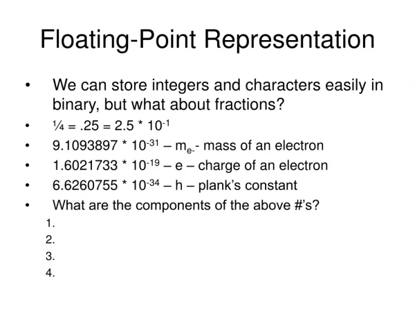
ECE 645: Lecture 2. Number Representation Part 2 Floating Point Representations Little-Endian vs. Big-Endian Representations Galois Field Representations. Required Reading. Behrooz Parhami, Computer Arithmetic: Algorithms and Hardware Design. Chapter 17, Floating-Point Representations.

E N D
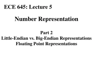
ECE 645: Lecture 2 Number Representation Part 2 Floating Point Representations Little-Endian vs. Big-Endian Representations Galois Field Representations
Required Reading Behrooz Parhami, Computer Arithmetic: Algorithms and Hardware Design Chapter 17, Floating-Point Representations Recommended Reading J-P. Deschamps, G. Bioul, G. Sutter, Synthesis of Arithmetic Circuits: FPGA, ASIC and Embedded Systems, Chapter 3.3, Real Numbers
Recommended Reading (to be covered at the next lecture) Behrooz Parhami, Computer Arithmetic: Algorithms and Hardware Design Chapter 5, Basic Addition and Counting J-P. Deschamps, G. Bioul, G. Sutter, Synthesis of Arithmetic Circuits: FPGA, ASIC and Embedded Systems, Chapter 4.1.1 Basic Algorithm Chapter 11.1 Basic AdderChapter 11.2 Carry-Chain Adder
The ANSI/IEEE standard floating-point number representation formats Originally IEEE 754-1985. Superseded by IEEE 754-2008 Standard.
Table 17.1 Some features of the ANSI/IEEE standard floatingpoint number representation formats
1.f 2e f = 0: Representation of f 0: Representation of NaNs f = 0: Representation of 0 f 0: Representation of denormals, 0.f 2–126 Exponent Encoding Exponent encoding in 8 bits for the single/short (32-bit) ANSI/IEEE format 0 1 126 127 128 254 255 Decimal code 00 01 7E 7F 80 FE FF Hex code Exponent value –126 –1 0 +1 +127
Rounding Modes The IEEE 754-2008 standard includes five rounding modes: Round to nearest, ties away from 0 (rtna) Round to nearest, ties to even (rtne) [default rounding mode] Round toward zero (inward) Round toward + (upward) Round toward – (downward)
rtna(x) Round to Nearest Number Rounding has a slight upward bias. Consider rounding (xk–1xk–2 ... x1x0.x–1x–2)two to an integer (yk–1yk–2 ... y1y0.)two The four possible cases, and their representation errors are: x–1x–2 Round Error 00 down 0 01 down –0.25 10 up 0.5 11 up 0.25 With equal prob., mean = 0.125 For certain calculations, the probability of getting a midpoint value can be much higher than 2–l Fig. 17.7 Rounding of a signed-magnitude value to the nearest number.
Directed Rounding: Motivation We may need result errors to be in a known direction Example: in computing upper bounds, larger results are acceptable, but results that are smaller than correct values could invalidate the upper bound This leads to the definition of directed rounding modes upward-directed rounding (round toward +) and downward-directed rounding (round toward –) (required features of IEEE floating-point standard)
Directed Rounding: Visualization Fig. 17.6 Truncation or chopping of a 2’s-complement number (same as downward-directed rounding). Fig. 17.12 Upward-directed rounding or rounding toward +.
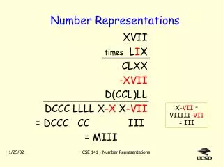
Exact result 1 + 2-1 + 2-23 + 2-24 Requirements for Arithmetic Results of the 4 basic arithmetic operations (+, -, , ) as well as square-rooting must match those obtained if all intermediate computations were infinitely precise That is, a floating-point arithmetic operation should introduce no more imprecision than the error attributable to the final rounding of a result that has no exact representation (this is the best possible) Example: (1 + 2-1) (1 + 2-23 ) Rounded result 1 + 2-1 + 2-22 Error = ½ ulp
New IEEE 754-2008 Standard Basic Formats
New IEEE 754-2008 Standard Binary Interchange Formats
Little-Endian vs. Big-Endian Representation of Integers
Little-Endian vs. Big-Endian Representation A0 B1 C2 D3 E4 F5 67 8916 MSB LSB Little-Endian Big-Endian 0 LSB = 89 MSB = A0 67 B1 F5 C2 E4 D3 address D3 E4 C2 F5 B1 67 MSB = A0 LSB = 89 MAX
Little-Endian vs. Big-Endian Camps 0 LSB MSB . . . . . . address MSB LSB MAX Little-Endian Big-Endian Motorola 68xx, 680x0 Bi-Endian Intel IBM AMD Motorola Power PC Hewlett-Packard DEC VAX Silicon Graphics MIPS Sun SuperSPARC RS 232 Internet TCP/IP
Little-Endian vs. Big-Endian Origin of the terms Jonathan Swift, Gulliver’s Travels • A law requiring all citizens of Lilliput to break their soft-eggs • at the little ends only • A civil war breaking between the Little Endians and • the Big-Endians, resulting in the Big Endians taking refuge on • a nearby island, the kingdom of Blefuscu • Satire over holy wars between Protestant Church of England • and the Catholic Church of France
Little-Endian vs. Big-Endian Advantages and Disadvantages Big-Endian Little-Endian • easier to determine a sign of • the number • easier to compare two numbers • easier to divide two numbers • easier to print • easier addition and multiplication • of multiprecision numbers
Pointers (1) Big-Endian Little-Endian 0 int * iptr; 89 (* iptr) = 8967; (* iptr) = 6789; 67 F5 E4 address iptr+1 D3 C2 B1 A0 MAX
Pointers (2) Big-Endian Little-Endian 0 long int * lptr; 89 (* lptr) = 8967F5E4; (* lptr) = E4F56789; 67 F5 E4 address D3 lptr + 1 C2 B1 A0 MAX
Polynomial Representation of the Galois Field elements
Evariste Galois (1811-1832) Studied the problem of finding algebraic solutions for the general equations of the degree 5, e.g., f(x) = a5x5+ a4x4+ a3x3+ a2x2+ a1x+ a0 = 0 Answered definitely the question which specific equations of a given degree have algebraic solutions On the way, he developed group theory, one of the most important branches of modern mathematics.
Evariste Galois (1811-1832) • Galois submits his results for the first time to • the French Academy of Sciences • Reviewer 1 • Augustin-Luis Cauchy forgot or lost the communication • 1830 Galois submits the revised version of his manuscript, • hoping to enter the competition for the Grand Prize • in mathematics • Reviewer 2 • Joseph Fourier – died shortly after receiving the manuscript • 1831 Third submission to the French Academy of Sciences • Reviewer 3 • Simeon-Denis Poisson – did not understand the manuscript • and rejected it.
Evariste Galois (1811-1832) • May 1832 Galois provoked into a duel • The night before the duel he writes a letter to his friend • containing the summary of his discoveries. • The letter ends with a plea: • “Eventually there will be, I hope, some people who • will find it profitable to decipher this mess.” • May 30, 1832 Galois is grievously wounded in the duel and dies • in the hospital the following day. • Galois manuscript rediscovered by Joseph Liouville • 1846 Galois manuscript published for • the first time in a mathematical journal
Field Set F, and two operations typically denoted by (but not necessarily equivalent to) + and * Set F, and definitions of these two operations must fulfill special conditions.
Examples of fields Infinite fields { R= set of real numbers, + addition of real numbers * multiplication of real numbers } Finite fields { set Zp={0, 1, 2, … , p-1}, + (mod p): addition modulo p, * (mod p): multiplication modulo p }
Quotient and remainder Given integers a and n, n>0 ! q, r Z such that a = q n + r and 0 r < n a q = q – quotient r – remainder (of a divided by n) = a div n n a r = a - q n = a – n = n = a mod n
mod 5 = • -32 mod 5 =
Integers coungruent modulo n Two integers a and b are congruent modulo n (equivalent modulo n) written a b iff a mod n = b mod n or a = b + kn, k Z or n | a - b
Rules of addition, subtraction and multiplication modulo n a + b mod n = ((a mod n) + (b mod n)) mod n a - b mod n = ((a mod n) - (b mod n)) mod n ab mod n = ((a mod n) (b mod n)) mod n
9 · 13 mod 5 = 25 · 25 mod 26 =
Laws of modular arithmetic Modular addition Regular addition a+ba+c (mod n) iff bc (mod n) a+b = a+c iff b=c Regular multiplication Modular multiplication If a b ac (mod n) and gcd(a, n) = 1 then bc (mod n) If a b = ac and a0 then b=c
Modular Multiplication: Example 18 42 (mod 8) 6 3 6 7 (mod 8) 3 7 (mod 8) 0 1 2 3 4 5 6 7 x 6 x mod 8 0 6 4 2 0 6 4 2 0 1 2 3 4 5 6 7 x 5 x mod 8 0 5 2 7 4 1 6 3
Sets of polynomials Z[x] - polynomials with coefficients in Z, e.g., f(x) = -4 x3 + 254 x2 + 45 x + 7 Zn[x] - polynomials with coefficients in Zn e.g., for n=15 f(x) = 3 x3 + 14 x2 + 4 x + 7 Z2[x] - polynomials with coefficients in Z2 e.g., f(x) = 1 x3 + 0 x2 + 1 x + 1 = x3 + x + 1