Part One: Introduction to Graphs
660 likes | 781 Vues
Explore relationship representations in economics through graph examples, variables, constants, and plotting on graphs. Learn x and y axes, coordinate points, and more.

Part One: Introduction to Graphs
E N D
Presentation Transcript
Part One: Introduction to Graphs
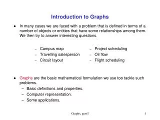
Mathematics and Economics • In economics many relationships are represented graphically. • Following examples demonstrate the types of skills you will be required to know and use in introductory economics courses.
An individual buyer's demand curve for corn • The law of demand: • Consumers will buy more of a product as its price declines.
Demand Curve for Paperback Books • Demand reflects an individual's willingness to buy various quantities of a good at various prices.
The concepts you will learn in this section are: • Constant vs. variable. • Dependent vs. independent variable. • x and y axes. • The origin on a graph. • x and y coordinates of a point. • Plot points on a graph.
Variables, Constants, andTheir Relationships • After reviewing this unit, you will be able to: • Define the terms constant and variable. • Identify whether an item is a constant or a variable. • Identify whether an item is a dependent or independent variable
Variables and Constants • Characteristics or elements such as prices, outputs, income, etc., are measured by numerical values. • The characteristic or element that remains the same is called a constant. • For example, the number of donuts in a dozen is a constant.
Some of these values can vary. • The price of a dozen donuts can change from $2.50 to $3.00. • We call these characteristics or elements variables.
Which of the following are variables and which are constants? • The temperature outside your house. • The number of square feet in a room that is 12 ft by 12 ft. • The noise level at a concert.
Relationships Between Variables • We express a relationship between two variables by stating the following: The value of the variable y depends upon the value of the variable x. • We can write the relationship between variables in an equation. • y = a + bx
The equation also has an "a" and "b" in it. • These are constants that help define the relationship between the two variables.
y = a + bx • In this equation the y variable is dependent on the values of x, a, and b. The y is the dependent variable. • The value of x, on the other hand, is independent of the values y, a, and b. The x is the independent variable.
An Example ... • A pizza shop charges 7 dollars for a plain pizza with no toppings and 75 cents for each additional topping added. • The total price of a pizza (y) depends upon the number of toppings (x) you order.
Price of a pizza is a dependent variable and number of toppings is the independent variable. • Both the price and the number of toppings can change, therefore both are variables.
The total price of the pizza also depends on the price of a plain pizza and the price per topping. • The price of a plain pizza and the price per topping do not change, therefore these are constants.
The relationship between the price of a pizza and the number of toppings can be expressed as an equation of the form: • y = a + bx
If we know that x (the number of toppings) and y (the total price) represent variables, what are a and b? • In our example, "a" is the price of a plain pizza with no toppings and "b" is the price of each topping. • They are constant.
We can set up an equation to show how the total price of pizza relates to the number of toppings ord
If we create a table of this particular relationship between x and y, we'll see all the combinations of x and y that fit the equation. For example, if plain pizza (a) is $7.00 and price of each topping (b) is $.75, we get: • y = 7.00 + .75x
Graphs • After reviewing this unit you will be able to: • Identify the x and y axes. • Identify the origin. on a graph. • Identify x and y coordinates of a point. • Plot points on a graph.
A graph is a visual representation of a relationship between two variables, x and y. • A graph consists of two axes called the x (horizontal) and y (vertical) axes. • The point where the two axes intersect is called the origin. The origin is also identified as the point (0, 0).
Coordinates of Points • A coordinate is one of a set of numbers used to identify the location of a point on a graph. • Each point is identified by both an x and a y coordinate.
Identifying the x-coordinate • Draw a straight line from the point directly to the x-axis. • The number where the line hits the x-axis is the value of the x-coord
Identifying the y-coordinate • Draw a straight line from the point directly to the y-axis. • The number where the line hits the axis is the value of the y-coordinate.
Notation for Identifying Points • Coordinates of point B are (100, 400) • Coordinates of point D are (400, 100)
Plotting Points on a Graph • Step One • First, draw a line extending out from the x-axis at the x-coordinate of the point. In our example, this is at 200.
Step Two • Then, draw a line extending out from the y-axis at the y-coordinate of the point. In our example, this is at 300.
Step Three • The point where these two lines intersect is at the point we are plotting, (200, 300).
Part Two: Equations and Graphs of Straight Lines
Economics and Linear Relationships • One of the most basic types of relationships is the linear relationship. • Many graphs in economics will display linear relationships, and you will need to use graphs to make interpretations about what is happening in a relationship.
Inverse relationship between ticket prices and game attendance • Two sets of data which are negatively or inversely related graph as a downsloping line. • The slope of this line is -1.25
Budget lines for $600 income with various prices for asparagus • As the price of asparagus rises, less and less can be purchased if the entire budget is spent on asparagus.
You will learn in this section to... • Draw a graph from a given equation. • Determine whether a given point lies on the graph of a given equation. • Define slope. • Calculate the slope of a straight line from its graph.
Be able to identify if a slope is positive, negative, zero, or infinite. • Identify the slope and y-intercept from the equation of a line. • Identify y-intercept from the graph of a line. • Match a graph with its equation.
Equations and Their Graphs • After reviewing this unit, you will be able to: • Draw a graph from a given equation. • Determine whether a given point lies on the graph of a given equation.
Graphing an Equation • Generate a list of points for the relationship. • Draw a set of axes and define the scale. • Plot the points on the axes. • Draw the line by connecting the points.
1. Generate a list of points for the relationship • In the pizza example, the equation is y = 7.00 + .75x. • You first select values of x you will solve for. • You then substitute these values into the equation and solve for they values.
2. Draw a set of axes and define the scale • Once you have your list of points you are ready to plot them on a graph. • The first step in drawing the graph is setting up the axes and determining the scale. • The points you have to plot are: • (0, 7.00), (1, 7.75), (2, 8.50), (3, 9.25), (4, 10.00)
Notice that the x values range from 0 to 4 and the y values go from 7 to 10. • The scale of the two axes must include all the points. • The scale on each axis can be different.
3. Plot the points on the axes • After you have drawn the axes, you are ready to plot the points. • Below we plot the points on a set of axes.
4. Draw the line by connecting the points • Once you have plotted each of the points, you can connect them and draw a straight line.
Checking a Point in the Equation • If, by chance, you have a point and you wish to determine if it lies on the line, you simply go through the same process as generating points. • Use the x value given in the point and insert it into the equation. • Compare the y value calculated with the one given in the point.
Example • Does point (6, 10) lie on the line y = 7.00 + .75x given in our pizza example? • To determine this, we need to plug the point (6, 10) into the equation. • The point with an x value of 6 that does lie on the line is (6, 11.5). • This means that the point (6, 10) does not lie on our line
Slope • After reviewing the unit you will be able to: • Define slope. • Calculate the slope of a straight line from its graph. • Identify if a slope is positive, negative, zero, or infinite. • Identify the slope and y-intercept from the equation of a line. • Identify the y-intercept from the graph of a line.
What is Slope? • The slope is used to tell us how much one variable (y) changes in relation to the change of another variable (x). • This can also be written in the form shown on the right.
As you may recall, a plain pizza with no toppings was priced at 7 dollars. • As you add one topping, the cost goes up by 75 cents.