Lecture 9 Feature Extraction and Motion Estimation
Lecture 9 Feature Extraction and Motion Estimation. Slides by : Michael Black Clark F. Olson Jean Ponce. Motion. Rather than using two cameras, we can extract information about the environment by moving a single camera. Some motion problems are similar to stereo: Correspondence

Lecture 9 Feature Extraction and Motion Estimation
E N D
Presentation Transcript
Lecture 9Feature Extraction and Motion Estimation Slides by: Michael Black Clark F. Olson Jean Ponce
Motion • Rather than using two cameras, we can extract information about the environment by moving a single camera. • Some motion problems are similar to stereo: • Correspondence • Reconstruction • New problem: motion estimation • Sometimes another problem is also present: • Segmentation: Which image regions correspond to rigidly moving objects.
Xj x1j x3j x2j P1 P3 P2 Structure From Motion Some textbooks treat motion largely from the perspective of small camera motions. We will not be so limited! • Given m pictures of n points, can we recover • the three-dimensional configuration of these points? • the camera configurations? (structure) (motion)
Structure From Motion Several questions must be answered: • What image points should be matched? • - feature selection • What are the correct matches between the images? • - feature tracking (unlike stereo, no epipolar constraint) • Given the matches, what is camera motion? • Given the matches, where are the points? Simplifying assumption: scene is static. • - objects don’t move relative to each other
Feature Selection We could track all image pixels, but this requires excessive computation. We want to select features that are easy to find in other images. Edges are easy to find in one direction, but not the other: aperture problem! Corner points (with gradients in multiple directions) can be precisely located.
“flat” region:no change in all directions “edge”:no change along the edge direction “corner”:significant change in all directions Corner Detection • We should easily recognize the point by looking through a small window. Shifting a window in anydirection should give a large change in intensity. Source: A. Efros
Corner Detection Basic idea for corner detection: • Find image patches with gradients in multiple directions. Input Corners selected 7
Corner Detection 2 x 2 matrix of image derivatives (averaged in neighborhood of a point). Notation:
Corner detection Classification of image points using eigenvalues of M: 2 “Edge” 2 >> 1 “Corner”1 and 2 are large,1 ~ 2;E increases in all directions 1 and 2 are small;E is almost constant in all directions “Edge” 1 >> 2 “Flat” region 1
Harris Corner Detector • Compute M matrix for each image window to get their cornernessscores. • Find points whose surrounding window gave large corner response. • Take the points of local maxima, i.e., perform non-maximum suppression.
Harris Corner Detector Input images
Harris Corner Detector Cornerness scores
Harris Corner Detector Thresholded
Harris Corner Detector Local maxima
Harris Corner Detector Corners output
Harris Detector Properties • Rotation invariant? • Scale invariant? Yes No All points will be classified as edges Corner !
Automatic Scale Selection • Intuition: • Find scale that gives local maxima of some function f in both position and scale.
Choosing a Detector • What do you want it for? • Precise localization in x-y: Harris • Good localization in scale: Difference of Gaussian • Flexible region shape: MSER • Best choice often application dependent • Harris-/Hessian-Laplace/DoG work well for many natural categories • MSER works well for buildings and printed things • Why choose? • Get more points with more detectors • There have been extensive evaluations/comparisons • [Mikolajczyk et al., IJCV’05, PAMI’05] • All detectors/descriptors shown here work well
Feature Tracking • Determining the corresponding features is similar to stereo vision. • Problem: epipolar lines unknown • - Matching point could be anywhere in the image. • If small motion between images, can search only in small neighborhood. • Otherwise, large search space necessary. • - Coarse-to-fine search used to reduce computation time.
Feature Tracking • Challenges: • Figure out which features can be tracked • Efficiently track across frames • Some points may change appearance over time (e.g., due to rotation, moving into shadows, etc.) • Drift: small errors can accumulate as appearance model is updated • Points may appear or disappear: need to be able to add/delete tracked points
Feature Matching Example: The set of vectors from each image location to the corresponding location in the subsequent image is called a motion field.
Feature Matching Example: If the camera motion is purely translation, the motion vectors all converge at the “focus-of-expansion”.
Ambiguity The relative position between the cameras has six degrees of freedom (six parameters): • - Translation in x, y, z • - Rotation about x, y, z Problem: images looks exactly the same if everything is scaled by a constant factor. For example: • - Cameras twice as far apart • - Scene twice as big and twice as far away Can only recover 5 parameters. • - Scale can’t be determined, unless known in advance
Structure From Motion • Given a set of corresponding points in two or more images, compute the camera parameters and the 3D point coordinates ? ? Camera 1 ? Camera 3 ? Camera 2 R1,t1 R3,t3 R2,t2 Slide credit: Noah Snavely
Solving for Structure and Motion Total number of unknown values: • - 5 camera motion parameters • - n point depths (where n is the number of points matched) Total number of equations: • - 2n (each point match has a constraint on the row and column) Can (in principle) solve for unknowns if 2n ≥ 5 + n (n ≥ 5) Usually, many more matches than necessary are used. • - Improves performance with respect to noise
Solving for Structure and Motion Once the motion is known, dense matching is possible using the epipolar constraint.
Multiple Images If there are more than two images, similar ideas apply: • - Perform matching between all images • - Use constraints given by matches to estimate structure and motion For m images and n points, we have: • - 6(m-1)-1+n unknowns = 6m-7+n • - 2(m-1)n constraints = 2mn-2n Can (in principle) solve when n is at least (6m-7)/(2m-3).
Bundle adjustment • Non-linear method for refining structure and motion • Minimizing reprojection error Xj P1Xj x3j x1j P3Xj P2Xj x2j P1 P3 P2
Stereo Ego-motion One application of structure from motion is to determine the path of a robot by examining the images that it takes. The use of stereo provides several advantages: • - The scale is known, since we can compute scene depths • - There is more information for matching points (depth)
Stereo Ego-motion Stereo ego-motion loop: • Feature selection in first stereo pair. • Stereo matching in first stereo pair. • Feature tracking into second stereo pair. • Stereo matching in second stereo pair. • Motion estimation using 3D feature positions. • Repeat with new images until done.
Ego-motion steps Features selected Features matched in right image Features tracked in left image Features tracked in right image
Stereo Ego-motion Odometry track Actual track (GPS) Estimated track “Urbie”
Advanced Feature Matching Right image Left image Left image after affine optimization