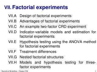
VII. Factorial experiments
VII. Factorial experiments. VII.A Design of factorial experiments VII.B Advantages of factorial experiments VII.C An example two-factor CRD experiment VII.D Indicator-variable m odels and estimation for factorial experiments

VII. Factorial experiments
E N D
Presentation Transcript
VII. Factorial experiments VII.ADesign of factorial experiments VII.B Advantages of factorial experiments VII.C An example two-factor CRD experiment VII.D Indicator-variable models and estimation for factorial experiments VII.E Hypothesis testing using the ANOVA method for factorial experiments VII.F Treatment differences VII.G Nested factorial structures VII.H Models and hypothesis testing for three-factor experiments Statistical Modelling Chapter VII
Factorial experiments • Often be more than one factor of interest to the experimenter. • Definition VII.1: Experiments that involve more than one randomized or treatment factor are called factorial experiments. • In general, the number of treatments in a factorial experiment is the product of the numbers of levels of the treatment factors. • Given the number of treatments, the experiment could be laid out as • a Completely Randomized Design, • a Randomized Complete Block Design or • a Latin Square with that number of treatments. • BIBDs or Youden Squares are not suitable. Statistical Modelling Chapter VII
VII.A Design of factorial experiments a) Obtaining a layout for a factorial experiment in R • Layouts for factorial experiments can be obtained in R using expressions for the chosen design when only a single-factor is involved. • Difference with factorial experiments is that the several treatment factors are entered. • Their values can be generated using fac.gen. • fac.gen(generate, each=1, times=1, order="standard") • It is likely to be necessary to use either the each or times arguments to generate the replicate combinations. • The syntax of fac.gen and examples are given in Appendix B, Randomized layouts and sample size computations in R. Statistical Modelling Chapter VII
Example VII.1 Fertilizing oranges • Suppose an experimenter is interested in investigating the effect of nitrogen and phosphorus fertilizer on yield of oranges. • Investigate 3 levels of Nitrogen (viz 0,30,60 kg/ha) and 2 levels of Phosphorus (viz. 0,20 kg/ha). • The yield after six months was measured. • Treatments are all possible combinations of the 3 Nitrogen 2 Phosphorus levels: 32 = 6 treatments. • The treatment combinations, arranged in standard order, are: Statistical Modelling Chapter VII
Specifies units indexed by Seedling with 18 levels. Creates 3 copies of the levels combinations of N and P, with 3 and 2 levels; stores these in the data.frameCRDFac2.ran. Does CRD randomization Remove excess objects Generating a layout in R for a CRD with 3 reps > # > # CRD > # > n <- 18 > CRDFac2.unit <- list(Seedling = n) > CRDFac2.ran <- fac.gen(list(N = c(0, 30, 60), P = c(0, 20)), times = 3) > CRDFac2.lay <- fac.layout(unrandomized = CRDFac2.unit, + randomized = CRDFac2.ran, seed = 105) > remove("CRDFac2.unit“, "CRDFac2.ran") Statistical Modelling Chapter VII
The layout > CRDFac2.lay Units Permutation Seedling N P 1 1 2 1 30 20 2 2 18 2 0 0 3 3 4 3 30 0 4 4 5 4 30 0 5 5 7 5 30 20 6 6 12 6 30 0 7 7 15 7 60 0 8 8 13 8 0 0 9 9 6 9 60 0 10 10 1 10 60 0 11 11 10 11 30 20 12 12 16 12 60 20 13 13 8 13 0 20 14 14 14 14 0 20 15 15 3 15 0 0 16 16 11 16 60 20 17 17 9 17 60 20 18 18 17 18 0 20 Statistical Modelling Chapter VII
What about an RCBD? • Suppose we decide on a RCBD with three blocks — how many units per block would be required? • Answer 6. • In factorial experiments not limited to two factors • Thus we may have looked at Potassium at 2 levels as well. How many treatments in this case? • Answer 322 =12. Statistical Modelling Chapter VII
VII.B Advantages of factorial experiments a) Interaction in factorial experiments • The major advantage of factorial experiments is that they allow the detection of interaction. • Definition VII.2: Two factors are said to interact if the effect of one, on the response variable, depends upon the level of the other. • If they do not interact, they are said to be independent. • To investigate whether two factors interact, the simple effects are computed. Statistical Modelling Chapter VII
Effects • Definition VII.3: A simple effect, for the means computed for each combination of at least two factors, is the difference between two of these means having different levels of one of the factors but the same levels for all other factors. • We talk of the simple effects of a factor for the levels of the other factors. • If there is an interaction, compute an interaction effect from the simple effects to measure the size of the interaction • Definition VII.4: An interaction effect is half the difference of two simple effects for two different levels of just one factor (or is half the difference of two interaction effects). • If there is not an interaction, can separately compute the main effects to see how each factor affects the response. • Definition VII.5: A main effect of a factor is the difference between two means with different levels of that factor, each mean having been formed from all observations having the same level of the factor. Statistical Modelling Chapter VII
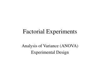
Example VII.2 Chemical reactor experiment • Investigate the effect of catalyst and temperature on the yield of chemical from a chemical reactor. • Table of means from the experimentwas as follows: • For A the temperature effect is 72-60 = 12 • For B the temperature effect is 64-52 = 12 • These are called the simple effects of temperature. • Clearly, the difference between (effect of) the temperatures is independent of which catalyst is used. • Interaction effect: [12 - 12]/2 = 0 Statistical Modelling Chapter VII
Illustrate using an interaction plot • A set of parallel lines indicates no interaction Statistical Modelling Chapter VII
Interaction & independence are symmetrical in factors • Thus, • the simple catalyst effect at 160°C is 52-60 =-8 • the simple catalyst effect at 180°C is 64-72 =-8 • Thus the difference between (effect of) the catalysts is independent of which temperature is used. • Interaction effect is still 0 and factors are additive. Statistical Modelling Chapter VII
Conclusion when independent • Can consider each factor separately. • Looking at overall means will indicate what is happening in the experiment. • So differences between the means in these tables are the main effects of the factors. • That is, the main effect of Temperature is 12 and that of Catalyst is -8. • Having used 2-way table of means to work out that there is no interaction, abandon it for summarizing the results. Statistical Modelling Chapter VII
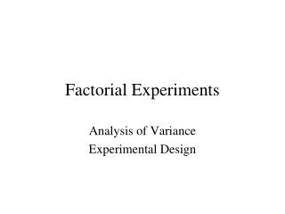
Example VII.3 Second chemical reactor experiment • Suppose results from experiment with 2nd reactor as follows: • The simple temperature effect for A is 72-60 = 12 • The simple temperature effect for B is 83-52 = 31 • Difference between (effect of) temperatures depends on which catalyst is used. • Statement symmetrical in 2 factors — say 2 factors interact. (also dependent or nonadditive) Statistical Modelling Chapter VII
Interaction plot • Clearly an interaction as lines have different slopes. • So cannot use overall means. Statistical Modelling Chapter VII
Why using overall means is inappropriate • Main effects: • cannot be equal to simple effects as these differ • have no practical interpretation. • Look at means for the combinations of the factors • Overall means are: • Interaction effect: • [(72-60) - (83-52)]/2 = [12 - 31]/2 = -9.5 • or [(52-60) - (83-72)]/2 = [-8 - 9]/2 = -9.5. • two non-interacting factors is the simpler Statistical Modelling Chapter VII
b) Advantages over one-factor-at-a-time experiments • Sometimes suggested better to keep it simple and investigate one factor at a time. • However, this is wrong. • Unable to determine whether or not there is an interaction. • Take temperature-catalyst experiment at 2nd reactor. • WELL YOU HAVE ONLY APPLIED THREE OF THE FOUR POSSIBLE COMBINATIONS OF THE TWO FACTORS • Catalyst A at 180°C has not been tested but catalyst B at 160°C has been tested twice as indicated above. Statistical Modelling Chapter VII
Limitation of inability to detect interaction • The results of the experiments would indicate that: • temperature increases yield by 31 gms • the catalysts differ by 8 gms in yield. • If we presume the factors act additively, predict the yield for catalyst A at 160°C to be: • 60+31 = 83 + 8 = 91. • This is quite clearly erroneous. • Need the factorial experiment to determine if there is an interaction. Statistical Modelling Chapter VII
Same resources but more info • Exactly the same total amount of resources are involved in the two alternative strategies, assuming the number of replicates is the same in all the experiments. • In addition, if the factors are additive then the main effects are estimated with greater precision in factorial experiments. • In the one-factor-at-a time experiments • the effect of a particular factor is estimated as the difference between two means each based on r observations. • In the factorial experiment • the main effects of the factors are the difference between two means based on 2r observations • which represents a sqrt(2) increase in precision. • The improvement in precision will be greater for more factors and more levels Statistical Modelling Chapter VII
Summary of advantages of factorial experiments if the factors interact, factorial experiments allow this to be detected and estimates of the interaction effect can be obtained, and if the factors are independent, factorial experiments result in the estimation of the main effects with greater precision. Statistical Modelling Chapter VII
VII.C An example two-factor CRD experiment • Modification of ANOVA: instead of a single source for treatments, will have a source for each factor and one for each possible combinations of factors. Statistical Modelling Chapter VII
a) Determining the ANOVA table for a two-Factor CRD • Description of pertinent features of the study • Observational unit • a unit • Response variable • Y • Unrandomized factors • Units • Randomized factors • A, B • Type of study • Two-factor CRD • The experimental structure Statistical Modelling Chapter VII
c) Sources derived from the structure formulae • Degrees of freedom and sums of squares • Units = Units • A*B =A + B + A#B • Hasse diagrams for this study with • degrees of freedom • M and Q matrices Statistical Modelling Chapter VII
e) The analysis of variance table Statistical Modelling Chapter VII
f) Maximal expectation and variation models • Assume the randomized factors are fixed and that the unrandomized factor is a random factor. • Then the potential expectation terms are A, B and AB. • The variation term is: Units. • The maximal expectation model is • y = E[Y] = AB • and the variation model is • var[Y] = Units Statistical Modelling Chapter VII
g) The expected mean squares • The Hasse diagrams, with contributions to expected mean squares, for this study are: Statistical Modelling Chapter VII
ANOVA table with E[MSq] Statistical Modelling Chapter VII
b) Analysis of an example Example VII.4 Animal survival experiment • To demonstrate the analysis I will use the example from Box, Hunter and Hunter (sec. 7.7). • In this experiment three poisons and four treatments (antidotes) were investigated. • The 12 combinations of poisons and treatments were applied to animals using a CRD and the survival times of the animals measured (10 hours). Statistical Modelling Chapter VII
A. Description of pertinent features of the study • These are the steps that need to be performed before R is used to obtain the analysis. • The remaining steps are left as an exercise for you. • Observational unit • an animal • Response variable • Survival Time • Unrandomized factors • Animals • Randomized factors • Treatments, Poisons • Type of study • Two-factor CRD • The experimental structure Statistical Modelling Chapter VII
Interaction plot • There is some evidence of an interaction in that the traces for each level of Treat look to be different. Statistical Modelling Chapter VII
Hypothesis test for the example Step 1: Set up hypotheses a) H0: there is no interaction between Poison and Treatment H1: there is an interaction between Poison and Treatment b) H0: r1=r2=r3 H1: not all population Poison means are equal c) H0: t1=t2=t3=t4 H1: not all population Treatment means are equal Set a= 0.05. Statistical Modelling Chapter VII
Hypothesis test for the example (continued) Step 2: Calculate test statistics • The ANOVA table for a two-factor CRD, with random factors being the unrandomized factors and fixed factors the randomized factors, is: Statistical Modelling Chapter VII
Hypothesis test for the example (continued) Step 3: Decide between hypotheses Interaction of Poison and Treatment is not significant, so there is no interaction. Both main effects are highly significant,so both factors affect the response. More about models soon. • Also, it remains to perform the usual diagnostic checking. Statistical Modelling Chapter VII
VII.D Indicator-variable models and estimation for factorial experiments • The models for the factorial experiments will depend on the design used in assigning the treatments — that is, CRD, RCBD or LS. • The design will determine the unrandomized factors and the terms to be included involving those factors. • They will also depend on the number of randomized factors. • Let the total number of observations be n and the factors be A and B with a and b levels, respectively. • Suppose that the combinations of A and B are each replicated r times — that is, n = abr. Statistical Modelling Chapter VII
a) Maximal model for two-factor CRD experiments • The maximal model used for a two-factor CRD experiment, where the two randomized factors A and B are fixed, is: where Y is the n-vector of random variables for the response variable observations, (ab)is the ab-vector of parameters for the A-B combinations, XABis the nab matrix giving the combinations of A and B that occurred on each unit, i.e. X matrix for AB, is the variability arising from different units. • Our model also assumes Y ~ N(yAB, V) Statistical Modelling Chapter VII
Standard order • Expression for X matrix in terms of direct products of Is and 1s when A and B are in standard order. • Previously used standard order — general definition in notes. • The values of the k factors A1, A2, …, Ak with a1, a2, …, ak levels, respectively, are systematically ordered in a hierarchical fashion: • they are ordered according to A1, then A2, then A3, … and then Ak. • Suppose, the elements of the Y vector are arranged so that the values of the factors A, B and the replicates are in standard order, as for a systematic layout. • Then Statistical Modelling Chapter VII
Then Example VII.5 22 Factorial experiment • Suppose A and B have 2 levels each and that each combination of A and B has 3 replicates. • Hence, a=b= 2, r= 3 and n= 12. • Then • Now Y is arranged so that the values of A, B and the reps are in standard order — that is • so that XAB for 4 level AB is: Statistical Modelling Chapter VII
Example VII.5 22 Factorial experiment (continued) • For the maximal model, • That is, the maximal model allows for a different response for each combination of A and B. Statistical Modelling Chapter VII
b) Alternative expectation models — marginality-compliant models Rule VII.1: The set of expectation models corresponds to the set of all possible combinations of potential expectation terms, subject to restriction that terms marginal to another expectation term are excluded from the model; • it includes the minimal model that consists of a single term for the grand mean. • For marginality of terms refer to Hasse diagrams and can be deduced using definition VI.9. • This definition states that one generalized factor is marginal to another if • the factors in the marginal generalized factor are a subset of those in the other and • this will occur irrespective of the replication of the levels of the generalized factors. Statistical Modelling Chapter VII
Two-factor CRD • For all randomized factors fixed, the potential expectation terms are A, B and AB. • Maximal model • includes all terms: E[Y] = A + B + AB • However, marginal terms must be removed • so the maximal model reduces to E[Y] = AB • Next model leaves out AB giving additive model E[Y] = A + B • no marginal terms in this model. • A simpler model than this is either E[Y] = A and E[Y] = B. • Only other possible model is one with neither A nor B: E[Y] = G. Statistical Modelling Chapter VII
Alternative expectation models in terms of matrices • Expressions for X matrices in terms of direct products of Is and 1s when A and B are in standard order. Statistical Modelling Chapter VII
X matrices • Again suppose, the elements of the Y vector are arranged so that the values of the factors A, B and the replicates are in standard order, as for a systematic layout. • Then the X matrices can be written as the following direct products: Statistical Modelling Chapter VII
Example VII.5 22 Factorial experiment (continued) • Remember A and B have two levels each and that each combination of A and B is replicated 3 times. • Hence, a = b = 2, r = 3 and n = 12. Then • Suppose Y is arranged so that the values of A, B and the replicates are in standard order — that is • Then Statistical Modelling Chapter VII
Example VII.5 22 Factorial experiment (continued) Notice, irrespective of the replication of the levels of AB , • XG can be written as a linear combination of the columns of each of the other three • XA and XB can be written as linear combinations of the columns of XAB. Statistical Modelling Chapter VII
Example VII.5 22 Factorial experiment (continued) • Marginality of indicator-variable terms (for generalized factors) • XGmXAa, XBb, XAB(ab). • XAa, XBbXAB(ab). • More loosely, for terms as seen in the Hasse diagram, we say that • G < A, B, AB • A, B < AB • Marginality of models (made up of indicator-variable terms) • yGyA, yB, yA+B, yAB[yG=XGm,yA=XAa, yB=XBb, yA+B=XAa + XBb, yAB=XAB(ab)] • yA, yByA+B, yAB[yA=XAa, yB=XBb,yA+B=XAa + XBb, yAB=XAB(ab)] • yA+ByAB[yA+B=XAa + XBb,yAB=XAB(ab)] • More loosely, • G < A, B, A+B, AB, • A, B < A+B, AB • A+B < AB. Statistical Modelling Chapter VII
are the n-vectors of means, the latter for the combinations of A and B, that is for the generalized factor AB. Estimators of the expected values for the expectation models • They are all functions of means. • So can be written in terms of mean operators, Ms. • If Y is arranged so that the associated factors A, B and the replicates are in standard order, the M operators written as the direct product of I and J matrices: Statistical Modelling Chapter VII
Example VII.5 22 Factorial experiment (continued) • The mean vectors, produced by an MY, are as follows: Statistical Modelling Chapter VII
VII.E Hypothesis testing using the ANOVA method for factorial experiments • Use ANOVA to choose between models. • In this section will use generic names of A, B and Units for the factors • Recall ANOVA for two-factor CRD. Statistical Modelling Chapter VII
a) Sums of squares for the analysis of variance • Require estimators of the following SSqs for a two-factor CRD ANOVA: • Total or Units; A; B; A#B and Residual. • Use Hasse diagram. Statistical Modelling Chapter VII
Vectors for sums of squares • All the Ms and Qs are symmetric and idempotent. Statistical Modelling Chapter VII