Download
1 / 25
250 likes | 274 Vues
Dive into Chapter 13 to learn how to perform statistical inference in regression analysis, focusing on the slope of the regression line. Explore hypothesis testing, confidence intervals, and prediction intervals in the context of regression models.

E N D
Chapter 13:Inference in Regression Lecture PowerPoint Slides
Chapter 13 Overview • 13.1 Inference About the Slope of the Regression Line • 13.2 Confidence Intervals and Prediction Intervals • 13.3 Multiple Regression
The Big Picture Where we are coming from and where we are headed… • In the later chapters of Discovering Statistics, we have been studying more advanced methods in statistical inference. • Here in Chapter 13, we return to regression analysis, first discussed in Chapter 4. At that time, we learned descriptive methods for regression analysis; now it is time to learn how to perform statistical inference in regression. • In the last chapter, we will explore nonparametric statistics.
13.1: Inference About the Slope of the Regression Line Objectives: • Explain the regression model and the regression model assumptions. • Perform the hypothesis test for the slope b1of the population regression equation. • Construct confidence intervals for the slope b1. • Use confidence intervals to perform the hypothesis test for the slope b1.
The Regression Model Recall that the regression line approximates the relationship between two continuous variables and is described by the regression equation y-hat= b1x + b0. Regression Model The population regression equation is defined as: where b0 is the y-intercept of the population regression line, b1 is the slope, and e is the error term. Regression Model Assumptions 1. Zero Mean: The error term is a random variable with mean = 0. 2. Constant Variance: The variance of e is the same regardless of the value of x. 3. Independence: The values of e are independent of each other. 4. Normality: The error term e is a normal random variable.
Hypothesis Tests for b1 To test whether there is a relationship between x and y, we begin with the hypothesis test to determine whether or not b1 equals 0. H0: b1 = 0 There is no linear relationship between x and y. Ha: b2 ≠ 0 There is a linear relationship between x and y. Test Statistic tdata where b1 represents the slope of the regression line represents the standard error of the estimate, and represents the numerator of the sample variance of the x data.
Hypothesis Tests for b1 H0: b1 = 0 There is no linear relationship between x and y. Ha: b2 ≠ 0 There is a linear relationship between x and y. Hypothesis Test for Slope b1 If the conditions for the regression model are met: Step 1: State the hypotheses. Step 2: Find the t critical value and the rejection rule. Step 3: Calculate the test statistic and p-value. Step 4: State the conclusion and the interpretation.
Example Ten subjects were given a set of nonsense words to memorize within a certain amount of time and were later scored on the number of words they could remember. The results are in Table 13.4. Test whether there is a relationship between time and score using level of significance a = 0.01. Note the graphs on page 640, indicating the conditions for the regression model have been met. H0: 1 = 0 There is no linear relationship between time and score. Ha: 1 ≠ 0 There is a linear relationship between time and score. Reject H0 if the p-value is less than a = 0.01.
Example Since the p-value of about 0.000 is less than a = 0.01, we reject H0. There is evidence for a linear relationship between time and score.
Confidence Interval for b1 Confidence Interval for Slope b1 When the regression assumptions are met, a 100(1 – a)% confidence interval for b1 is given by: where t has n – 2 degrees of freedom. Margin of Error The margin of error for a 100(1 – a)% confidence interval for b1 is given by: As in earlier sections, we may use a confidence interval for the slope to perform a two-tailed test for b1. If the interval does not contain 0, we would reject the null hypothesis.
13.2: Confidence Intervals and Prediction Intervals Objectives: • Construct confidence intervals for the mean value of y for a given value of x. • Construct prediction intervals for a randomly chosen value of y for a given value of x.
Confidence Interval for the Mean Value of y for a Given x Confidence Interval for the Mean Value of y for a Given x A (100 – a)% confidence interval for the mean response, that is, for the population mean of all values of y, given a value of x, may be constructed using the following lower and upper bounds: where x* represents the given value of the predictor variable. The requirements are that the regression assumptions are met or the sample size is large.
Prediction Interval for an Individual Value of y for a Given x Prediction Interval for an Individual Value of y for a Given x A (100 – a)% confidence interval for a randomly selected value of y given a value of x may be constructed using the following lower and upper bounds: where x* represents the given value of the predictor variable. The requirements are that the regression assumptions are met or the sample size is large.
13.3: Multiple Regression Objectives: • Find the multiple regression equation, interpret the multiple regression coefficients, and use the multiple regression equation to make predictions. • Calculate and interpret the adjusted coefficient of determination. • Perform the F test for the overall significance of the multiple regression. • Conduct t tests for the significance of individual predictor variables. • Explain the use and effect of dummy variables in multiple regression. • Apply the strategy for building a multiple regression model.
Multiple Regression Thus far, we have examined the relationship between the response variable y and a single predictor variable x. In our data-filled world, however, we often encounter situations where we can use more than one x variable to predict the y variable. Multiple regression describes the linear relationship between one response variable y and more than one predictor variable x1, x2, …. The multiple regression equation is an extension of the regression equation where k represents the number of x variables in the equation and b0, b1, … represent the multiple regression coefficients. The interpretation of the regression coefficients is similar to the interpretation of the slope in simple linear regression, except that we add that the other x variables are held constant.
Adjusted Coefficient of Determination We measure the goodness of a regression equation using the coefficient of determination r2= SSR/SST. In multiple regression, we use the same formula for the coefficient of determination (though the letter r is promoted to a capital R). Multiple Coefficient of Determination R2 The multiple coefficient of determination is given by: R2= SSR/SST 0 ≤ R2≤ 1 where SSR is the sum of squares regression and SST is the total sum of squares. The multiple coefficient of determination represents the proportion of the variability in the response y that is explained by the multiple regression equation.
Adjusted Coefficient of Determination Unfortunately, when a new x variable is added to the multiple regression equation, the value of R2 always increases, even when the variable is not useful for predicting y. So, we need a way to adjust the value of R2 as a penalty for having too many unhelpful x variables in the equation. Adjusted Coefficient of Determination R2adj The adjusted coefficient of determination is given by: where n is the number of observations, k is the number of x variables, and R2is the multiple coefficient of determination.
F Test for Multiple Regression The multiple regression model is an extension of the model from Section 13.1, and approximates the relationship between y and the collection of x variables. Multiple Regression Model The population multiple regression equation is defined as: where b1, b2,…,bkare the parameters of the population regression equation, k is the number of x variables, and e is the error term that follows a normal distribution with mean 0 and constant variance. The population parameters are unknown, so we must perform inference to learn about them. We begin by asking: Is our multiple regression useful? To answer this, we perform the F test for the overall significance of the multiple regression.
F Test for Multiple Regression The hypotheses for the F test are: H0: b1 = b2 = … =bk = 0 Ha: At least one of the b’s ≠ 0. The F test is not valid if there is strong evidence that the regression assumptions have been violated. F Test for Multiple Regression If the conditions for the regression model are met Step 1: State the hypotheses and the rejection rule. Step 2: Find the F statistic and the p-value. (Located in the ANOVA table of computer output.) Step 3: State the conclusion and the interpretation.
t Test for Individual Predictor Variables To determine whether a particular x variable has a significant linear relationship with the response variable y, we perform the t test that was used in Section 13.1 to test for the significance of that x variable. t Test for Individual Predictor Variables One may perform as many t tests as there are predictor variables in the model, which is k. If the conditions for the regression model are met: Step 1: For each hypothesis test, state the hypotheses and the rejection rule. Step 2: For each hypothesis test, find the t statistic and the p-value. Step 3: For each hypothesis test, state the conclusion and the interpretation.
Dummy Variables It is possible to include binomial categorical variables in multiple regression by using a “dummy variable.” A dummy variable is a predictor variable used to recode a binomial categorical variable in regression by taking values 0 or 1. Recoding the multiple regression equation will result in two different regression equations, one for one value of the categorical variable and one for the other. These two regression equations will have the same slope, but different y-intercepts.
Building a Multiple Regression Model Strategy for Building a Multiple Regression Model Step 1:The F Test – Construct the multiple regression equation using all relevant predictor variables. Apply the F test in order to make sure that a linear relationship exists between the response y and at least one of the predictor variables. Step 2:The t Tests – Perform the t tests for the individual predictors. If at least one of the predictors is not significant, then eliminate the x variable with the largest p-value from the model. Repeat until all remaining predictors are significant. Step 3:Verify the Assumptions – For your final model, verify the regression assumptions. Step 4: Report and Interpret Your Final Model – Provide the multiple regression equation, interpret the multiple regression coefficients, and report and interpret the standard error of the estimate and the adjusted coefficient of determination.
Chapter 13 Overview • 13.1 Inference About the Slope of the Regression Line • 13.2 Confidence Intervals and Prediction Intervals • 13.3 Multiple Regression