Download
1 / 35
360 likes | 703 Vues
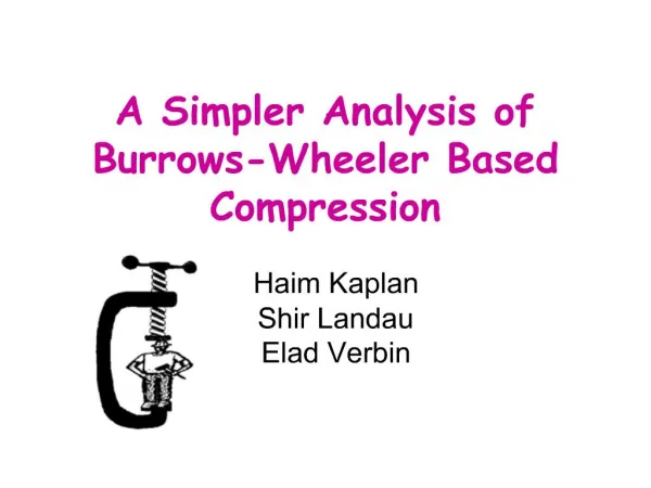
A Simpler Analysis of Burrows-Wheeler Based Compression. Haim Kaplan Shir Landau Elad Verbin . Our Results. Improve the bounds of one of the main BWT based compression algorithms New technique for worst case analysis of BWT based compression algorithms using the Local Entropy

E N D
A Simpler Analysis of Burrows-Wheeler Based Compression Haim Kaplan Shir Landau Elad Verbin
Our Results • Improve the bounds of one of the main BWT based compression algorithms • New technique for worst case analysis of BWT based compression algorithms using the Local Entropy • Interesting results concerning compression of integer strings
The Burrows-Wheeler Transform(1994) Given a string S the Burrows-Wheeler Transform creates a permutation of S that is locally homogeneous. S BWT S’ is locally homogeneous
Empirical Entropy - Intuition The Problem – Given a string S encode each symbol in S using a fixed codeword…
Example: Huffman Code 1 0 0 1 1 0 0 1 Order-0 Entropy (Shannon 48) H0(s): Maximum compression we can get using only frequencies and no context information
Context 1 for s “isis” Context 1 for i “mssp” Order-k entropy Hk(s): Lower bound for compression with order-k contexts – the codeword representing each symbol depends on the k symbols preceding it MISSISSIPPI Traditionally, compression ratio of compression algorithms measured using Hk(s)
String S BWT Burrows-Wheeler Transform MTF Move-to-front ? RLE Run-Length encoding Order-0 Encoding Compressed String S’ History The Main Burrows-Wheeler Compression Algorithm (Burrows, Wheeler 1994):
a b a c a b a c a b b b b c a c c c d d d d d d MTF Given a string S = baacb over alphabet = {a,b,c,d} S = b a a c b MTF(S) = 1 1 0 2 2
Main Bounds (Manzini 1999) • gk is a constant dependant on the context k and the size of the alphabet • these are worst-case bounds
Some Intuition… • H0 – “measures” frequency • Hk – “measures” frequency and context → We want a statistic that measures local similarity in a string and specifically in the BWT of the string
Some Intuition… • The more the contexts are similar in the original string, the more its BWT will exhibit local similarity… • The more local similarity found in the BWT of the string the smaller the numbers we get in MTF… → The solution: Local Entropy
MTF Original string Integer sequence The Local Entropy- Definition We define: given a string s = “s1s2…sn” The local entropy of s: (Bentley, Sleator, Tarjan, Wei, 86)
The Local Entropy - Definition Note: LE(s) = number of bits needed to write the MTF sequence in binary. Example: MTF(s)= 311 → LE(s) = 4 → MTF(s) in binary = 1111 In Dream world… We would like to compress S to LE(S)…
The Local Entropy – Properties We use two properties of LE: • The entropy hierarchy • Convexity
The Local Entropy – Property 1 • The entropy hierarchy: We prove: For each k: LE(BWT(s)) ≤ nHk(s) + O(1) → Any upper bound that we get for BWT with LE holds for Hk(s) as well.
The Local Entropy – Properties 2 • Convexity: → This means that a partition of a string s does not improve the Local Entropy of s.
a b a a a b a b Convexity • Cutting the input string into parts doesn’t influence much: Only positions per part
String S BWT Burrows-Wheeler transform Booster RHC Variation of Huffman encoding Partition of BWT(S) BWT(S) Compressed String S’ Convexity – Why do we need it? Ferragina, Giancarlo, Manzini and Sciortino, JACM 2005:
Using LE and its properties we get our bounds Theorem: For every where Our LE bound Our Hk bound
Our bounds We get an improvement of the known bounds: As opposed to the known bounds (Manzini, 1999):
Our Test Results *The files are non-binary files from the Canterbury corpus. gzip results are also taken from the corpus. The size is indicated in bytes.
How is LE related to compression of integer sequences? • We mentioned “dream world” but what about reality? How close can we come to ? Problem: Compress an integer sequence S close to its sum of logs: Notice for any s:
Compressing Integer Sequences • Universal Encodings of Integers: prefix-free encoding for integers (e.g. Fibonacci encoding). • Doing some math, it turns out that order-0 encoding is good. Not only good: It is best!
The order-0 math • Theorem: For any string s of length n over the integer alphabet {1,2,…h} and for any , • Strange conclusion… we get an upper-bound on the order-0 algorithm with a phrase dependant on the value of the integers. • This is true for all strings but is especially interesting for strings with smaller integers.
A lower bound for SL Theorem: For any algorithm A and for any , and any C such that C < log(ζ(μ)) there exists a string S of length n for which: |A(S)| > μ∙SL(S) + C∙n
Our Results - Summary • New improved bounds for BWMTF • Local Entropy (LE) • New bounds for compression of integer strings
? Open Issues We question the effectiveness of . Is there a better statistic?
Thank You! Italy France Anybody want to guess??
Creating a Huffman encoding • For each encoding unit (letter, in this example), associate a frequency (number of times it occurs) • Create a binary tree whose children are the encoding units with the smallest frequencies • The frequency of the root is the sum of the frequencies of the leaves • Repeat this procedure until all the encoding units are in the binary tree
Example • Assume that relative frequencies are: • A: 40 • B: 20 • C: 10 • D: 10 • R: 20
Assign 0 to left branches, 1 to right branches Each encoding is a path from the root Example, cont. A = 0B = 100C = 1010D = 1011R = 11
a nana# b b anana # Sort the rows n a#ban a n ana#b a The Burrows-Wheeler Transform The Burrows-Wheeler Transform (1994) Given a string S = banana# banana# # banan a anana#b a #banan nana#ba a na#ba n ana#ban na#bana a#banan #banana
So all we need to get the BWT is the suffix array! #banan a a#banan anana#b ana#ba n b anana # na#ban a nana#b a Suffix Arrays and the BWT The Suffix Array Index of BWT 7 6 4 2 1 5 3 6 5 3 1 7 4 2