Turbulent Heating of the Solar Wind at 1 AU

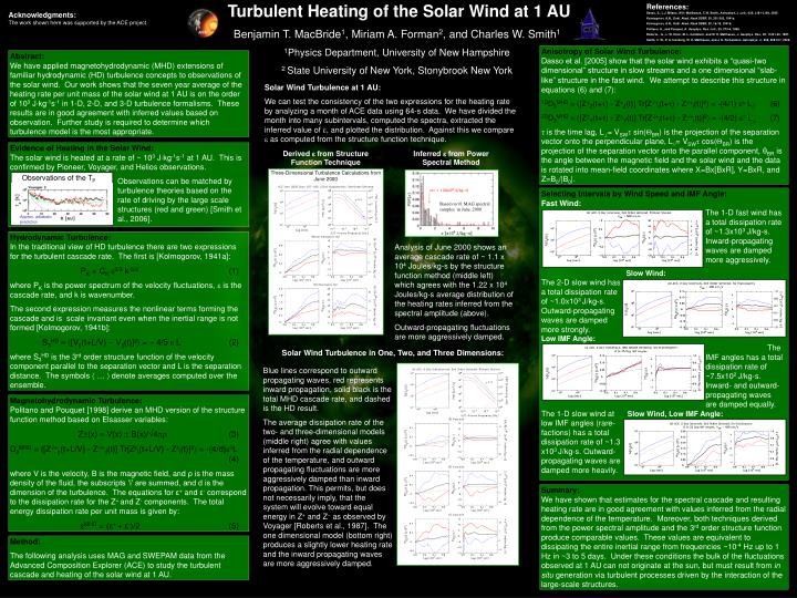
1. Turbulent Heating of the Solar Wind at 1 AU Observations of the TP Three-Dimensional Turbulence Calculations from June 2000 Based on 91 MAG spectral samples in June, 2000 Approx. adiabatic prediction References: Dasso, S., L.J. Milano, W.H. Matthaeus, C.W. Smith, Astrophys. J. Lett., 635, L181-L184, 2005. Kolmogorov, A.N., Dokl. Akad. Nauk SSSR, 30, 301-305, 1941a. Kolmogorov, A.N., Dokl. Akad. Nauk SSSR, 32, 16-18, 1941b. Politano, H., and Pouquet, A. Geophys. Res. Lett., 25, 273-6, 1998. Roberts, . A., L. W. Klein, M. L. Goldstein, and W. H. Matthaeus, J. Geophys. Res., 92, 11021-40, 1987. Smith, C. W., P. A. Isenberg, W. H. Matthaeus, and J. D. Richardson, Astrophys. J., 638, 508-517, 2006. Acknowledgments: The work shown here was supported by the ACE project. Benjamin T. MacBride1, Miriam A. Forman2, and Charles W. Smith1 1Physics Department, University of New Hampshire 2 State University of New York, Stonybrook New York Anisotropy of Solar Wind Turbulence:Dasso et al. [2005] show that the solar wind exhibits a “quasi-two dimensional” structure in slow streams and a one dimensional “slab-like” structure in the fast wind.We attempt to describe this structure in equations (6) and (7): 1DD3MHD  [ZZ(t+) - ZZ(t)] Tr[Z-/+i(t+) - Z-/+i(t)]2 = -(4/1)  L (6) 2DD3MHD  [ZY(t+) - ZY(t)] Tr[Z-/+i(t+) - Z-/+i(t)]2 = -(4/2)  L (7)  is the time lag, L= VSW sin(BR) is the projection of the separation vector onto the perpendicular plane, L= VSW cos(BR) is the projection of the separation vector onto the parallel component, θBR is the angle between the magnetic field and the solar wind and the data is rotated into mean-field coordinates where X=Bx[BxR], Y=BxR, and Z=B0/|B0|. Abstract:We have applied magnetohydrodynamic (MHD) extensions of familiar hydrodynamic (HD) turbulence concepts to observations of the solar wind.Our work shows that the seven year average of the heating rate per unit mass of the solar wind at 1 AU is on the order of 103 Jkg-1s-1 in 1-D, 2-D, and 3-D turbulence formalisms. These results are in good agreement with inferred values based on observation. Further study is required to determine which turbulence model is the most appropriate. Solar Wind Turbulence at 1 AU: We can test the consistency of the two expressions for the heating rate by analyzing a month of ACE data using 64-s data. We have divided the month into many subintervals, computed the spectra, extracted the inferred value of , and plotted the distribution. Against this we compare  as computed from the structure function technique. Evidence of Heating in the Solar Wind:The solar wind is heated at a rate of ~ 103 Jkg-1s-1 at 1 AU. This is confirmed by Pioneer, Voyager, and Helios observations. Observations can be matched by turbulence theories based on the rate of driving by the large scale structures (red and green) [Smith et al., 2006]. Derived  from Structure Function Technique Inferred  from Power Spectral Method Selecting Intervals by Wind Speed and IMF Angle: Fast Wind: The 1-D fast wind has a total dissipation rate of ~1.3x103 J/kg-s. Inward-propagating waves are damped more aggressively. Slow Wind: The 2-D slow wind has a total dissipation rate of ~1.0x103J/kg-s. Outward-propagating waves are damped more strongly. Low IMF Angle: The 1-D wind at low IMF angles has a total dissipation rate of ~7.5x102J/kg-s. Inward- and outward- propagating waves are damped equally. The 1-D slow wind at Slow Wind, Low IMF Angle: low IMF angles (rare-factions) has a totaldissipation rate of ~1.3x103 J/kg-s. Outward-propagating waves are damped more heavily. Inertial range spectrum is f-5/3. Hydrodynamic Turbulence:In the traditional view of HD turbulence there are two expressions for the turbulent cascade rate. The first is [Kolmogorov, 1941a]: PK = CK2/3k-5/3 (1) where PK is the power spectrum of the velocity fluctuations,  is the cascade rate, and k is wavenumber. The second expression measures the nonlinear terms forming the cascade and is scale invariant even when the inertial range is not formed [Kolmogorov, 1941b]: S3HD [V||(t+L/V)  V||(t)]3 =  4/5  L (2) where S3HDis the 3rd order structure function of the velocity component parallel to the separation vector and L is the separation distance. The symbols  …  denote averages computed over the ensemble. Analysis of June 2000 shows an average cascade rate of ~ 1.1 x 104 Joules/kg-s by the structure function method (middle left) which agrees with the 1.22 x 104 Joules/kg-s average distribution of the heating rates inferred from the spectral amplitude (above). Outward-propagating fluctuations are more aggressively damped. Solar Wind Turbulence in One, Two, and Three Dimensions: Blue lines correspond to outward propagating waves, red represents inward propagation, solid black is the total MHD cascade rate, and dashed is the HD result. The average dissipation rate of the two- and three-dimensional models (middle right) agree with values inferred from the radial dependence of the temperature, and outward propagating fluctuations are more aggressively damped than inward propagation. This permits, but does not necessarily imply, that the system will evolve toward equal energy in Z+ and Z as observed by Voyager [Roberts et al., 1987]. The one dimensional model (bottom right) produces a slightly lower heating rate and the inward propagating waves are more aggressively damped. Magnetohydrodynamic Turbulence:Politano and Pouquet [1998] derive an MHD version of the structure function method based on Elsasser variables: Z(x)  V(x)  B(x)/4 (3) D3MHD  [Z-/+||(t+L/V) - Z-/+||(t)] Tr[Zi(t+L/V) - Zi(t)]2 = -(4/d)L (4) where V is the velocity, B is the magnetic field, and ρ is the mass density of the fluid, the subscripts ‘i’ are summed, and d is the dimension of the turbulence. The equations for ε+ and ε- correspond to the dissipation rate for the Z+ and Z- components. The total energy dissipation rate per unit mass is given by: εMHD = (ε+ + ε-)/2 (5) Summary:We have shown that estimates for the spectral cascade and resulting heating rate are in good agreement with values inferred from the radial dependence of the temperature. Moreover, both techniques derived from the power spectral amplitude and the 3rd order structure function produce comparable values. These values are equivalent to dissipating the entire inertial range from frequencies ~10-4 Hz up to 1 Hz in ~3 to 5 days. Under these conditions the bulk of the fluctuations observed at 1 AU can not originate at the sun, but must result from in situ generation via turbulent processes driven by the interaction of the large-scale structures. Method: The following analysis uses MAG and SWEPAM data from the Advanced Composition Explorer (ACE) to study the turbulent cascade and heating of the solar wind at 1 AU.