Download
1 / 46
470 likes | 569 Vues
Explore the complex origins of the solar wind, from magnetic connectivity to turbulence in the corona, with insights on energy transport and heating mechanisms. Discover the mysteries behind fast and slow solar winds and the role of magnetic fields. Uncover the challenges of measuring coronal bis and the dynamics of flux tubes. Delve into global magnetic field connectivity and the dissipation of magnetic energy along flux tubes. Dive into the intricate interplay of location, energy dissipation, and acceleration of solar wind.

E N D
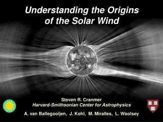
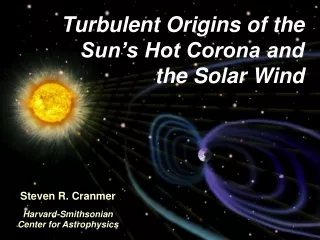
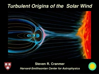
Turbulent Origins of the Solar Wind Steven R. CranmerHarvard-Smithsonian Center for Astrophysics
Outline: 1. A tour of magnetic connectivity & plasma properties: wind corona chromosphere photosphere 2. Energy transport: turbulent coronal heating “recipe” Turbulent Origins of the Solar Wind Steven R. CranmerHarvard-Smithsonian Center for Astrophysics
Overview: the solar atmosphere Heating is everywhere!
fast slow speed (km/s) Tp (105 K) Te (105 K) Tion / Tp O7+/O6+, Mg/O 600–800 2.4 1.0 > mion/mp low 300–500 0.4 1.3 < mion/mp high In situ solar wind: properties • Mariner 2 (1962): first direct confirmation of continuous fast & slow solar wind. • Uncertainties about which type is “ambient” persisted because measurements were limited to the ecliptic plane . . . • Ulysses left the ecliptic; provided 3D view of the wind’s source regions. By ~1990, it was clear the fast wind needs something besides gas pressure to accelerate so fast!
Wang et al. (2000) In situ solar wind: connectivity • High-speed wind: strong connections to the largest coronal holes hole/streamer boundary (streamer “edge”) streamer plasma sheet (“cusp/stalk”) small coronal holes active regions • Low-speed wind: still no agreement on the full range of coronal sources:
Wind Speed Expansion Factor Coronal magnetic fields • Coronal Bis notoriously difficult to measure . . . • Potential field source surface (PFSS) models have been successful in reproducing observed structures and mapping between Sun & in situ. • Wang & Sheeley (1990) flux-tube expansion correlation, modified by, e.g., Arge & Pizzo (2000).
Coronal magnetic fields: solar minimum A(r) ~ B(r)–1 ~ r2f(r) Banaszkiewicz et al. (1998)
SUPERSONIC coronal heating: subsonic region is unaffected. Energy flux has nowhere else to go: M same, u vs. SUBSONIC coronal heating: “puffs up” scale height, draws more particles into wind: M u Why is the fast/slow wind fast/slow? • Several ideas exist; one powerful one relates the spatial dependence of the heating to the location of the Parker critical point; this determines how the “available” heating affects the plasma (e.g., Leer & Holzer 1980): Banaszkiewicz et al. (1998)
Wind origins in open magnetic regions • UV spectroscopy shows blueshifts in supergranular network (e.g., Hassler et al. 1999) Leighton (1963)
Supergranular “funnels” Peter (2001) Fisk (2005) Tu et al. (2005)
Inter-granular bright points (close-up) • It’s widely believed that the G-band bright points are strong-field (1500 G) flux tubes surrounded by much weaker-field plasma. 100–200 km
splitting/merging torsion longitudinal flow/wave bending (kink-mode wave) Waves in thin flux tubes • Statistics of horizontal BP motions gives power spectrum of “kink-mode” waves. • BPs undergo both random walks & intermittent (reconnection?) “jumps:”
splitting/merging torsion longitudinal flow/wave bending (kink-mode wave) Waves in thin flux tubes • Statistics of horizontal BP motions gives power spectrum of “kink-mode” waves. • BPs undergo both random walks & intermittent (reconnection?) “jumps:” In reality, it’s not just the “pure” kink mode. . . (Hasan et al. 2005)
Global magnetic field connectivity • Cranmer & van Ballegooijen (2005) built a model of the global properties of incompressible non-WKB Alfvenic turbulence along an open flux tube. • Lower boundary condition: observed horizontal motions of G-band bright points. • Along the flux tube, wave/turbulence properties should be computed consistently.
How is magnetic energy dissipated along these open flux tubes? How does this energy get into the corona to heat & accelerate the solar wind?
Coronal heating: “location location location” • The basal coronal heating problem is well known: • Above 2 Rs , additional energy deposition is required in order to . . . • accelerate the fast solar wind (without artificially boosting mass loss and peak Te ), • produce the proton/electron temperatures seen in situ (also the varying magnetic moment!), • produce the strong preferential heating and temperature anisotropy of heavy ions (in the wind’s acceleration region) seen with UV spectroscopy.
UVCS/SOHO: fast solar wind • In coronal holes, heavy ions (e.g., O+5) both flow faster and are heated hundreds of times more strongly than protons and electrons, and have anisotropic temperatures. (e.g., Kohl et al. 1997, 1998, 2006)
Heating mechanisms • A surplus of proposed ideas? (Mandrini et al. 2000; Aschwanden et al. 2001)
Heating mechanisms • A surplus of proposed ideas? (Mandrini et al. 2000; Aschwanden et al. 2001) • Where does the mechanical energy come from? vs.
Heating mechanisms • A surplus of proposed ideas? (Mandrini et al. 2000; Aschwanden et al. 2001) • Where does the mechanical energy come from? • How is this energy coupled to the coronal plasma? vs. waves shocks eddies (“AC”) twisting braiding shear (“DC”) vs.
Heating mechanisms • A surplus of proposed ideas? (Mandrini et al. 2000; Aschwanden et al. 2001) • Where does the mechanical energy come from? • How is this energy coupled to the coronal plasma? • How is the energy dissipated and converted to heat? vs. waves shocks eddies (“AC”) twisting braiding shear (“DC”) vs. interact with inhomog./nonlin. turbulence reconnection collisions (visc, cond, resist, friction) or collisionless
Heating mechanisms • A surplus of proposed ideas? (Mandrini et al. 2000; Aschwanden et al. 2001) • Where does the mechanical energy come from? • How is this energy coupled to the coronal plasma? • How is the energy dissipated and converted to heat? vs. waves shocks eddies (“AC”) twisting braiding shear (“DC”) vs. interact with inhomog./nonlin. turbulence reconnection collisions (visc, cond, resist, friction) or collisionless
MHD turbulence • It is highly likely that somewhere in the outer solar atmosphere the fluctuations become turbulent and cascade from large to small scales:
MHD turbulence • It is highly likely that somewhere in the outer solar atmosphere the fluctuations become turbulent and cascade from large to small scales: • With a strong background field, it is easier to mix field lines (perp. to B) than it is to bend them (parallel to B). • Also, the energy transport along the field is far from isotropic: Z– Z+ Z– (e.g., Matthaeus et al. 1999; Dmitruk et al. 2002)
A recipe for coronal heating? Ingredients: • “Outer scale” correlation length (L): flux tube width (Hollweg 1986), normalized to something like 100 km at the photosphere. • Z+ and Z– : need to solve non-WKB Alfven wave reflection equations. refl. coeff = |Z+|2/|Z–|2
Alfven waves: non-WKB reflection, turbulent damping, wave-pressure acceleration • Acoustic waves: shock steepening, TdS & conductive damping, full spectrum, wave-pressure acceleration • Rad. losses: transition from optically thick (LTE) to optically thin (CHIANTI + PANDORA) • Heat conduction: transition from collisional (electron & neutral H) to collisionless “streaming” Turbulent heating models • Cranmer & van Ballegooijen (2005) solved the wave equations & derived heating rates for a fixed background state. • New models: (preliminary!) self-consistent solution of waves & background one-fluid plasma state along a flux tube: photosphere to heliosphere • Ingredients:
Turbulent heating models • For a polar coronal hole flux-tube: • Basal acoustic flux: 108 erg/cm2/s (equiv. “piston” v = 0.3 km/s) • Basal Alfvenic perpendicular amplitude: 0.4 km/s • Basal turbulent scale: 120 km (G-band bright point size!) T (K) reflection coefficient Transition region is too high (8 Mm instead of 2 Mm), but otherwise not bad . . .
Why is the fast/slow wind fast/slow? • Compare multiple 1D models in solar-minimum flux tubes with Ulysses 1st polar pass(Goldstein et al. 1996):
Why is the fast/slow wind fast/slow? • Compare multiple 1D models in solar-minimum flux tubes with Ulysses 1st polar pass(Goldstein et al. 1996): “Geometry is destiny?”
Progress toward a robust recipe Not too bad, but . . . • Because of the need to determine non-WKB (nonlocal!) reflection coefficients, it may not be easy to insert into global/3D MHD models. • Doesn’t specify proton vs. electron heating (they conduct differently!) • Probably doesn’t work for loops (keep an eye on Marco Velli) • Are there additional (non-photospheric) sources of waves / turbulence / heating for open-field regions? (e.g., flux cancellation events) (B. Welsch et al. 2004)
More plasma diagnostics Better understanding! Conclusions • Theoretical advances in MHD turbulence are continuing to “feed back” into global models of the solar wind. • High-resolution adaptive-optics studies of photospheric flux tubes pay off as the “bottom boundary condition” to coronal heating! • SOHO (especially UVCS) has led to fundamentally new views of the extended acceleration regions of the solar wind. • For more information: • http://cfa-www.harvard.edu/~scranmer/ SOHO: 1995–20??
The solar wind • 1958: Gene Parker proposed that the hot corona provides enough gas pressure to counteract gravity and accelerate a “solar wind.” 1962: Mariner 2 confirmed it! • Momentum conservation: To sustain a wind, /t = 0, and RHS must be naturally “tuned:” Cranmer (2004), Am. J. Phys.
UVCS / SOHO • SOHO (the Solar and Heliospheric Observatory) was launched in Dec. 1995 with 12 instruments probing solar interior to outer heliosphere. • The Ultraviolet Coronagraph Spectrometer (UVCS) measures plasma properties of coronal protons, ions, and electrons between 1.5 and 10 solar radii. • Combines occultation with spectroscopy to reveal the solar wind acceleration region. slit field of view: • Mirror motions select height • Instrument rolls indep. of spacecraft • 2 UV channels: LYA & OVI • 1 white-light polarimetry channel
On-disk profiles: T = 1–3 million K Off-limb profiles: T > 200 million K ! UVCS results: solar minimum (1996-1997) • The fastest solar wind flow is expected to come from dim “coronal holes.” • In June 1996, the first measurements of heavy ion (e.g., O+5) line emission in the extended corona revealed surprisingly wide line profiles . . .
The impact of UVCS UVCS has led to new views of the collisionless nature of solar wind acceleration. Key results include: • The fast solar wind becomes supersonic much closer to the Sun (~2 Rs) than previously believed. • In coronal holes, heavy ions (e.g., O+5) both flow faster and are heated hundreds of times more strongly than protons and electrons, and have anisotropic temperatures. (e.g., Kohl et al. 1997,1998)
Spectroscopic diagnostics • Off-limb photons formed by both collisional excitation/de-excitation and resonant scattering of solar-disk photons. • Profile width depends on line-of-sight component of velocity distribution (i.e., perp. temperature and projected component of wind flow speed). • Total intensity depends on the radial component of velocity distribution (parallel temperature and main component of wind flow speed), as well as density. • If atoms are flow in the same direction as incoming disk photons, “Doppler dimming/pumping” occurs.
Doppler dimming & pumping • After H I Lyman alpha, the O VI 1032, 1037 doublet are the next brightest lines in the extended corona. • The isolated 1032 line Doppler dims like Lyman alpha. • The 1037 line is “Doppler pumped” by neighboring C II line photons when O5+ outflow speed passes 175 and 370 km/s. • The ratio R of 1032 to 1037 intensity depends on both the bulk outflow speed (of O5+ ions) and their parallel temperature. . . • The line widths constrain perpendicular temperature to be > 100 million K. • R < 1 implies anisotropy!
Coronal holes: over the solar cycle • Even though large coronal holes have similar outflow speeds at 1 AU (>600 km/s), their acceleration (in O+5) in the corona is different! (Miralles et al. 2001, 2004) Solar minimum: Solar maximum:
Alfven wave’s oscillating E and B fields ion’s Larmor motion around radial B-field Ion cyclotron waves in the corona • UVCS observations have rekindled theoretical efforts to understand heating and acceleration of the plasma in the (collisionless?) acceleration region of the wind. • Ion cyclotron waves (10 to 10,000 Hz) suggested as a natural energy source that can be tapped to preferentially heat & accelerate heavy ions. • Dissipation of these waves produces diffusion in velocity space along contours of ~constant energy in the frame moving with wave phase speed: lower Z/A faster diffusion
freq. horiz. wavenumber horiz. wavenumber something else? But does turbulence generate cyclotron waves? • Preliminary models say “probably not” in the extended corona. (At least not in a straightforward way!) • In the corona, “kinetic Alfven waves” with high k heat electrons (T >> T ) when they damp linearly. How then are the ions heated & accelerated? • Nonlinear instabilities that locally generate high-freq. waves (Markovskii 2004)? • Coupling with fast-mode waves that do cascade to high-freq. (Chandran 2006)? • KAW damping leads to electron beams, further (Langmuir) turbulence, and Debye-scale electron phase space holes, which heat ions perpendicularly via “collisions” (Ergun et al. 1999; Cranmer & van Ballegooijen 2003)? cyclotron resonance-like phenomena MHD turbulence
Alfven wave amplitude (with damping) • Cranmer & van Ballegooijen (2005) solved transport equations for 300 discrete periods (3 sec to 3 days), then renormalized using photospheric power spectrum. • One free parameter: base “jump amplitude” (0 to 5 km/s allowed; 3 km/s is best)
Turbulent heating rate • Solid curve: predicted Qheat for a polar coronal hole. • Dashed RGB regions: empirical estimates of heating rate of primary plasma (models tuned to match conditions at 1 AU). • What is really needed are direct measurements of the plasma (atoms, ions, electrons) in the acceleration region of the solar wind!
Streamers with UVCS • Streamers viewed “edge-on” look different in H0 and O+5 • Ion abundance depletion in “core” due to grav. settling? • Brightest “legs” show negligible outflow, but abundances consistent with in situ slow wind. • Higher latitudes and upper “stalk” show definite flows (Strachan et al. 2002). • Stalk also has preferential ion heating & anisotropy, like coronal holes! (Frazin et al. 2003)
The Need for Better Observations • Even though UVCS/SOHO has made significant advances, • We still do not understand the physical processes that heat and accelerate the entire plasma (protons, electrons, heavy ions), • There is still controversy about whether the fast solar wind occurs primarily in dense polar plumes or in low-density inter-plume plasma, • We still do not know how and where the various components of the variable slow solar wind are produced (e.g., “blobs”). (Our understanding of ion cyclotron resonance is based essentially on just one ion!) UVCS has shown that answering these questions is possible, but cannot make the required observations.