Advancements in Sequence Alignment Algorithms in Computational Biology
This presentation delves into the critical role of sequence alignment algorithms in computational biology, focusing on the Needleman-Wunsch and Smith-Waterman algorithms. These methods are essential for comparing DNA, RNA, and protein sequences, helping to identify homologous proteins, predict structures, and locate regulatory elements. The content covers scoring functions, alignment examples, and discusses the time and space complexities involved. Understanding these concepts is crucial for bioinformaticians aiming to analyze and interpret biological sequence data effectively.

Advancements in Sequence Alignment Algorithms in Computational Biology
E N D
Presentation Transcript
Sequence Alignment Algorithms in Computational Biology Spring 2006 Edited by Itai Sharon Most slides have been created and edited by Nir Friedman, Dan Geiger, Shlomo Moran and Ydo Wexler
Sequence Comparison • Much of bioinformatics involves sequences • DNA sequences • RNA sequences • Protein sequences • We can think of these sequences as strings of letters • DNA & RNA: alphabet ∑of 4 letters • Protein: alphabet ∑ of 20 letters
Sequence comparison: Motivation Finding similarity between sequences is important for many biological questions. • Find homologous proteins • Allows to predict structure and function • Locate similar subsequences in DNA • e.g: allows to identify regulatory elements • Locate DNA sequences that might overlap • Helps in sequence assembly
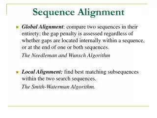
Sequence Alignment • Input: two sequences over the same alphabet • Output: an alignment of the two sequences • Two basic variants of sequence alignment: • Global – all characters in both sequences participate • Needleman-Wunsch, 1970 • Local – find related regions within sequences • Smith-Waterman, 1981
Sequence Alignment - Example • Input: GCGCATGGATTGAGCGAandTGCGCCATTGATGACCA • Possible output: -GCGC-ATGGATTGAGCGA TGCGCCATTGAT-GACC-A • Three elements: • Perfect matches • Mismatches • Insertions & deletions (indel)
Scoring Function • Score each position independently: • Match: +1 • Mismatch: -1 • Indel: -2 • Score of an alignment is sum of position scores • Example: -GCGC-ATGGATTGAGCGA TGCGCCATTGAT-GACC-A Score: (+1x13) + (-1x2) + (-2x4) = 3 ------GCGCATGGATTGAGCGA TGCGCC----ATTGATGACCA-- Score: (+1x5) + (-1x6) + (-2x11) = -23
Sequence vs. Structure Similarity Sequence 1 lcl|1A6M:_ MYOGLOBIN Length 151 (1..151) Sequence 2 lcl|1JL7:A MONOMER HEMOGLOBIN COMPONENT III Length 147 (1..147) Score = 31.6 bits (70), Expect = 10 Identities = 33/137 (24%), Positives = 55/137 (40%), Gaps = 17/137 (12%) Query: 2 LSEGEWQLVLHVWAKVEA--DVAGHGQDILIRLFKSHPETLEKFDRFKHLKTEAEMKASE 59 LS + Q+V W + + AG G++ L + +HPE F + Sbjct: 2 LSAAQRQVVASTWKDIAGADNGAGVGKECLSKFISAHPEMAAVFG--------FSGASDP 53 Query: 60 DLKKHGVTVLTALGAI---LKKKGHHEAELKPLAQSH---ATKHKIPIKYLEFISEAIIH 113 + + G VL +G L +G AE+K + H KH I +Y E + +++ Sbjct: 54 GVAELGAKVLAQIGVAVSHLGDEGKMVAEMKAVGVRHKGYGNKH-IKAEYFEPLGASLLS 112 Query: 114 VLHSRHPGDFGADAQGA 130 + R G A A+ A Sbjct: 113 AMEHRIGGKMNAAAKDA 129
Sequence vs. Structure Similarity 1A6M: Myoglobin 1JL7: Hemoglobin
Global Alignment • Input: two sequences over the same alphabet • Output: an alignment of the two sequences in which all characters in both sequences participate • The Needleman-Wunsch algorithm finds an optimal global alignment between two sequences • Uses a scoring function • A dynamic programming algorithm
The Needleman-Wunsch (NW) Algorithm • Suppose we have two sequences: • s=s1…sn and t=t1…tm • Construct a matrix V[n+1, m+1] in which V(i, j) contains the score for the best alignment between s1…si and t1…tj. • The grade for cell V(i, j) is: V(i-1, j)+score(si, -) V(I, j) = max V(i, j-1)+score(-, tj) V(i-1, j-1)+score(si, tj) • V(n,m) is the score for the best alignment between s and t
NW Algorithm – An Example • Alphabet: • DNA, ∑ = {A,C,G,T} • Input: • s = AAAC • t = AGC • Scoring scheme: • score(x, x) = 1 • score(x,-) = -2 • score(x, y) = -1
-4 -6 -2 -3 -4 -2 -6 -3 -2 -8 -5 -4 NW Algorithm – An Example -AGC AAAC 0 -2 1 -1 AG-C AAAC -1 0 -1 A-GC AAAC -1
-4 -6 -2 -3 -4 -2 -6 -3 -2 -8 -5 -4 NW – Time and Space Complexity Time: • Filling the matrix: • Backtracing: • Overall: Space: • Holding the matrix: 0 -2 O(n·m) O(n+m) 1 -1 O(n·m) -1 0 -1 O(n·m) -1
NW – Space Complexity • In real-life applications, n and m can be very large • The space requirements of O(n·m) can be too demanding • If n = m = 1000 we need O(1MB) space • If n = m = 10000 we need O(100MB) space • We can afford to perform extra computation to save space • Looping over million operations takes less than seconds on modern workstations • Can we trade space with time?
A G C 0 -2 -4 -6 A -2 1 -1 -3 A -4 -1 0 -2 A -6 -3 -2 -1 C -8 -5 -4 -1 Why Do We Need So Much Space? • We can do the same computation in O(min(n,m)) space: • Compute V(i, j) column by column, storing only two columns in memory (or row by row if rows are shorter). • However… • Trace back information requires O(m·n) memory bytes.
Space Efficient Version • Input: sequences s=s1…sn and t=t1…tm to be aligned. • Idea: perform divide and conquer • find position (i, n/2) at which some best alignment crosses a midpoint • Construct alignments A=s1…sn/2 vs. t=t1…ti and B=sn/2+1…sn vs. t=ti+1…tm • Return AB s t
Finding a Midpoint • The score of the best alignment that goes through i equals: score(s1…sn/2, t1…ti) + score(sn/2+1…sn, ti+1…tm) • Thus, we need to compute these two quantities for all values of i
Finding a Midpoint • Define • F(i, j) = score(s1…si, t1…ti) • B(i, j) = score(si+1…sn, tj+1…tm) • F(i, j) + B(i, j) = score of best alignment through (i, j) • Compute F(i, j) and B(i, j) in linear space complexity • We compute F(i, j) in O(min(i, j)) • We compute B(i, j) in exactly the same manner, going “backward” from B(n,m)
Time Complexity • Time to find a mid-point: c·n·m (c - a constant) • Size of recursive sub-problems is (n/2,i) and (n/2,m-i), hence: T(n,m) = c·n·m + T(n/2,i) + T(n/2,m-i) • Lemma: T(n, m) 2c·n·m • Proof: T(n,m) c·n·m + 2c(n/2)i + 2c(n/2)(m-i) = 2c·n·m.