Download
1 / 40
420 likes | 728 Vues
AY202a Galaxies & Dynamics Lecture 7: Jeans’ Law, Virial Theorem Structure of E Galaxies. Jean’s Law. Star/Galaxy Formation is most simply defined as the process of going from hydrostatic equilibrium to gravitational collapse.

E N D
AY202a Galaxies & DynamicsLecture 7: Jeans’ Law, Virial TheoremStructure of E Galaxies
Jean’s Law Star/Galaxy Formation is most simply defined as the process of going from hydrostatic equilibrium to gravitational collapse. There are a host of complicating factors --- left for a graduate course: Rotation Cooling Magnetic Fields Fragmentation ……………
The Simple Model Mc Assume a spherical, isothermal gas cloud that starts near Rc hydrostatic equlibrium: 2K + U = 0 (constant density) ρo Rc Tc Spherical Gas Cloud
Rc 0 3 GMc2 Potential Energy U =∫ -4πG M(r) ρ(r) r dr ~ - Mc = Cloud Mass Rc = Cloud Radius ρ0 = constant density = 5 Rc Mc 4/3 π Rc3
The Kinetic Energy, K, is just K = 3/2 N k T where N is the total number of particles, N = MC /(μ mH) where μ is the mean molecular weight and mH is the mass of Hydrogen The condition for collapse from the Virial theorem (more later) is 2 K < |U|
3 MC kT 3G MC2 < μ mH 5 RC So collapse occurs if and substituting for the cloud radius, We can find the critical mass for collapse: MC > MJ ~ ( ) ( ) 3 MC 1/3 RC = ( ) 4πρ0 5 k T 3 3/2 1/2 G μ mH 4 πρ0
If the cloud’s mass is greater than MJ it will collapse. Similarly, we can define a critical radius, RJ, such that if a cloud is larger than that radius it will collapse: RC> RJ ~( ) and note that these are of course for ideal conditions. Rotation, B, etc. count. 1/2 15 k T 4 π G μ mHρ0
Mass Estimators: The simplest case = zero energy bound orbit. Test particle in orbit, mass m, velocity v, radius R, around a body of mass M E = K + U = 1/2 mv2 - GmM/R = 0 1/2 mv2 = GmM/R M = 1/2 v2 R /G This formula gets modified for other orbits (i.e. not zero energy) e.g. for circular orbits 2K + U = 0 so M = v2 R /G What about complex systems of particles?
The Virial Theorem Consider a moment of inertia for a system of N particles and its derivatives: I = ½ Σ mi ri . ri (moment of inertia) I = dI/dt = Σ mi ri . ri I = d2I/dt2 = Σ mi (ri . ri + ri . ri ) N i=1 . . . . .. ..
Assume that the N particles have mi and ri and are self gravitating --- their mass forms the overall potential. We can use the equation of motion to elimiate ri : miri = -Σ ( ri - rj ) and note that Σmiri . ri = 2T (twice the Kinetic Energy) .. .. Gmimj |ri –rj|3 j = i . .
.. Gmi mj Then we can write (after substitution) I – 2T = -ΣΣ ri. (ri – rj) = -ΣΣ rj. (rj – ri) = - ½ ΣΣ (ri - rj).(ri – rj) = - ½ ΣΣ = U the potential energy |ri - rj|3 i j=i Gmi mj reversing labels |rj - ri|3 j i=j Gmi mj adding |ri - rj|3 i j=i Gmi mj |ri - rj|
.. I = 2T + U If we have a relaxed (or statistically steady) systemwhich is not changing shape or size, d2I/dt2 = I = 0 • 2T + U = 0; U = -2T; E = T+U = ½ U conversely, for a slowly changing or periodic system 2 <T> + <U> = 0 .. Virial Equilibrium
Virial Mass Estimator We use the Virial Theorem to estimate masses of astrophysical systems (e.g. Zwicky and Smith and the discovery of Dark Matter) Go back to: Σ mi<vi2> = ΣΣGmimj < > where < > denotes the time average, and we have N point masses of mass mi, position ri and velocity vi N N 1 |ri – rj| i=1 i=1 j<i
Assume the system is spherical. The observables are (1) the l.o.s. time average velocity: < v2R,i>Ω = 1/3 vi2 projected radial v averaged over solid angle i.e. we only see the radial component of motion & vi ~ √3 vr Ditto for position, we see projected radii R, R = θd , d = distance, θ = angular separation
1 1 1 So taking the average projection, < >Ω = < >Ω and <>Ω = = = π/2 Remember we only see 2 of the 3 dimensions with R |ri – rj| sin θij |Ri – Rj| ∫0πdθ ∫(sinθ)-1dΩ 1 sin ij ∫π0sinθdθ dΩ
Thus after taking into account all the projection effects, and if we assume masses are the same so that Msys = Σ mi = N mi we have MVT = N this is the Virial Theorem Mass Estimator Σ vi2 = Velocity dispersion [Σ (1/Rij)]-1 = Harmonic Radius Σ vi2 3π Σ (1/Rij) 2G i<j i<j
This is a good estimator but it is unstable if there exist objects in the system with very small projected separations: x x x x x xx x x x x x x x x x x x x x x all the potential energy is in this pair!
Projected Mass Estimator In the 1980’s, the search for a stable mass estimator led Bahcall & Tremaine and eventually Heisler, Bahcall & Tremaine to posit a new estimator with the form ~ [dispersion x size ]
Derived PM Mass estimator checked against simulations: MP = Σ vi2 Ri,c where Ri,c = Projected distance from the center vi = l.o.s. difference from the center fp = Projection factor which depends on (includes) orbital eccentricities fp GN
The projection factor depends fairly strongly on the average eccentricities of the orbits of the objects (galaxies, stars, clusters) in the system: fp = 64/π for primarily Radial Orbits = 32/π for primarily Isotropic Orbits = 16/π for primarily Circular Orbits (Heisler, Bahcall & Tremaine 1985) Richstone and Tremaine plotted the effect of eccentricity vs radius on the velocity dispersion profile:
Expected projected l.o.s. sigmas Richstone & Tremaine
Applications: Coma Cluster (PS2) M31 Globular Cluster System σ ~ 155 km/s MPM = 3.1+/-0.5 x 1011 MSun Virgo Cluster (core only!) σ ~ 620 km/s MVT = 7.9 x 10¹⁴ MSun MPM = 8.9 x 10¹⁴ MSun Etc.
M31 Globular Clusters (Perrett et al.)
The Structure of Elliptical Galaxies Main questions 1. Why do elliptical galaxies have the shapes they do? 2. What is the connection between light & mass & kinematics? = How do stars move in galaxies? Basic physical description: star piles. For each star we have (r, , ) or (x,y,z) and (dx/dt, dy/dt, dz/dt) = (vx,vy,vz) the six dimensional kinematical phase space Generally treat this problem as the motion of stars (test particles) in smooth gravitational potentials
For the system as a whole, we have the density, ρ(x,y,z) or ρ(r,,) The Mass M = ∫ ρ dV The Gravitational (x) = -G ∫ d3x’ Potential Force on unit mass at x F(x) = - (x) plus Energy Conservation Angular Momentum Conservation Mass Conservation (orthogonally) ρ(x’) |x’-x|
Plus Poisson’s Equation: 2 = 4 πGρ (divergence of the gradient) Gauss’s Theorem 4 π G ∫ρ dV = ∫ d2S enclose mass surface integral For spherical systems we also have Newton’s theorems: 1. A body inside a spherical shell sees no net force 2. A body outside a closed spherical shell sees a force = all the mass at a point in the center. The potential = -GM/r
G M(r) r The circular speed is then vc2 = r d/dr = and the escape velocity from such a potential is ve = 2 | (r) | ~ 2 vc For homogeneous spheres with ρ = const r rs = 0 r > rs vc = ( )1/2r 4πGρ 3
We can also ask what is the “dynamical time” of such a system the Free Fall Time from the surface to the center. Consider the equation of motion = - = - r Which is a harmonic oscillator with frequency 2π/T where T is the orbital peiod of a mass on a circular orbit T = 2πr/vc = (3π/Gρ)1/2 d2r GM(r) 4πGρ dt2 r2 3
3π 16 G ρ Thus the free fall time is ¼ of the period td = ( )½ The problem for most astrophysical systems reduces to describing the mass density distribution which defines the potential. E.g. for a Hubble Law, if M/L is constant I(r) = I0/(a + r)2 = I0a-2/(1 + r/a)2 so ρ(r) [(1 + r/a)2]-3/2 ρ0[(1 + r/a)2]-3/2
A distributions like this is called a Plummer model --- density roughly constant near the center and falling to zero at large radii For this model = - By definition, there are many other possible spherical potentials, one that is nicely integrable is the isochrone potential GM r2 + a2 - GM (r) = b + b2 +r2
Today there are a variety of “two power” density distributions in use ρ(r) = With = 4 these are called Dehnen models = 4, α = 1 is the Hernquist model = 4, α = 2 is the Jaffe model = 3, α = 1 is the NFW model ρ0 (r/a)α(1 – r/a)-α
Circular velocities versus radius Mod Hubble law Dehnen like laws
Theory’s End There is a theory which states that if ever anyone discovers exactly what the Universe is for and why it is here, it will instantly disappear and be replaced by something even more bizzare and inexplicable. There is another theory which states that this has already happened. Douglas Adams