Download
1 / 38
380 likes | 532 Vues
AY202a Galaxies & Dynamics Lecture 8: Structure of E Galaxies. Isothermal Spheres. Classic simple model: isotropic velocity distribution, collision-less stars, Polytropic index n = ∞ P = K ρ ((n+1)/n) = K ρ

E N D
AY202a Galaxies & DynamicsLecture 8: Structure of E Galaxies
Isothermal Spheres Classic simple model: isotropic velocity distribution, collision-less stars, Polytropic index n = ∞P = K ρ((n+1)/n) = Kρ Describe this model in terms of the hydrostatic equilibrium of an isothermal gas where K = Boltzmann’s constant T = temperature M = mass/particle dP kT dρ - ρ GM(r) = = dr m dr r2
d d ln ρ Gm dr dr kT and ( r2 ) = -4 π r2ρ(r) If the phase space density (energy) of the stars is Maxwell Boltzmann: f(E) = e –E/σ2 then Poisson’s Equation is ( r2 ) = -4 π G r2 ρ(r)/σ2 andσ2= kT/mprovides the definitionof T ρ (2πσ2)3/2 d d ln ρ dr dr
Isothermal Spheres BT
An isothermal gas sphere is identical to a collisionless system of stars with f(E) as above The Velocity distribution is a Maxwellian F(V) = N e - ½ v2/σ2 (elastic Maxwell Boltzmann dist) this model gives so ρ ∞ as r 0 feh! σ2 ρ(r) = 2π G r2
Solution to this problem was developed by Ivan King in his studies of the kinematics of globular clusters. Rescale ρ =ρ/ρ0 r = r/r0 then r0 = ( ) ½ ≡ core radius add a tidal cutoff and we have “softened” and “truncated” models, ρ 0 at r t, characterized by a concentration index c = log ( rt / r0) or by (0)/σ2 = central potential / velocity dispersion 9 σ2 4π G ρ0
King Profiles Potential Surface Mass density
King Models shape vs c
NGC3379 rc rt
Non-Spherical Models Ellipsoidal bodies solved in gory detail by Chandrasekhar. Result from Rotation but also Anisotropic Dispersion Fields (Tensors) Equilibrium Spheroids Jacobi Ellipsoids MacLaurin Spheres Reimann Ellipsoids Kuzmin, Toomre Disks General Triaxial Systems
Start with some definitions --- Isodensity surfaces of regular ellipsoids (bx)2 + (by)2 + z2 = a2 b > 1 prolate or cigar shaped b < 1 oblate or saucer shaped These are axisymmetric systems Triaxial systems have (cx)2 + (by)2 + z2 = a2 So the game is to solve Laplace’s equation 2 = 0 in oblate spherical coordinates
First transform from normal cylindrical coords (R, z, ) to oblate spherical coordinates (u,v, ) stays as the azimuthal angle and R = Δ cosh(u) sin(v), z = sinh(u) cos(v) Δ is a random constant Curves of constant u are confocal ellipses with foci at (R,z) = (±Δ,0) After much algebra = A [π/2 – arcsin(sech(u)) + Ψ0] where A and Ψ0 are constants. p.s. prolate a pain!
For large u, sech(u) 0, so • ≈ A(π/2 + Ψ0 – sech(u)) ≈ A(π/2 + Ψ0 +Δ/r) where r is our normal spherical variable r. We want 0 at ∞ and not singular at r = 0 So we can set Ψ0 = - ½ π, A = GM/Δ and the resulting potential is = x Everywhere continuous, 0 at ∞, u0 is a “core radius” - GM arcsin(sech(u0)) for u < u0 Δ arcsin(sech(u)) for u ≥ u0
This potential is that of a shell on u0 where the shell with u=u0 has dimensions semimajor axis a = Δ cosh u0 semiminor axis b = Δ sinh u0 so its ecccentrcity e = (1-b2/a2)½ = sech u0 and = x - GM arcsin(e) for u < u0 Δ arcsin(sech(u)) for u ≥ u0
Generalized Triaxial Systems 3 x1, x2, x3 constant m2 = a12 where the ai are constants (major, minor, subminor axes) The potential is constant of ellipsoidal surfaces constant = m2 = a12 xi2 a i2 i=1 3 xi2 ai2 + τ i=1
∞ a2 a3 [Ψ(∞ )-Ψ(m)] dτ Then the potential is (x,y,z) = -πG( ) ∫ where Ψ(m) = ∫ ρ(m2) dm2 is the integral of the mass density. • How do stars move in these potentials? • Can stars define the average potential? (Chandrasekhar) a1 √(τ+a1)2(τ+a2)2(τ+a3)2 0 m
Effective Potential for Rotating Axisymmetric Ellipsoids Lz2 eff = (r,z) + = ½ vo2 ln (r2 + z2/q2) + q = axial ratio Some Solutions: Box Orbits Loop Orbits Radial Orbits Tube Orbits 2r2 Lz2 2r2
Consider the potential (x,y) = ½ v02 ln (rc2 + x2 + y2/q2) q 1 Box Orbits – star passes through every point in a rectangular box r << rc Loop Orbits r >> rc
q = 0.9 q = 0.5 BT
Round Flat BT
Two orbits in the potential of equation 3-50 with q=0.9. Both orbits have energy E=-0.8 and angular momentum Lz = 0.2
One of the most eccentric loop orbits and one of the most elongated box orbits in the potential q = 0.9 Rc = 0.14
This has lead to the description of E systems in terms of the superposition of 3 types of orbits: Circular Radial Isotropic Orbits can be prograde or retrograde so L can be anything! One can even get “Boxy” versus “Disky” galaxies
Boxy NGC4731 Disky NGC1300 Contopoulous ‘88; Costa & Fitzgibbons; England ‘89
Rotation in Ellipticals Now we can describe them in terms of the Tensor Virial Theorem Potential Energy Tensor Kinetic Energy Tensor TVT balances potential energy tensor with the kinetic energy tensor. Wjk = - ∫ ρ(x) xj (∂/∂xk) d3x Kjk = ½ ∫ ρ(x) vj vk d3x
Kjk can be split into ordered and random terms Kjk = Tjk + ½ Πjk where Tjk = ½ ∫ρvj vk d3x Πjk = ∫ ρσ2jk d3x The moment of inertia tensor is Ijk = ∫ ρxj xkd3x differentiating ½ d2 Ijk /dt2 = 2 Tjk+Πjk + Wjk the Tensor Virial Theorem
If I is not time dependent Scalar Virial Theorem 2K + W = 0 Rotating Ellipticals 2Txx = ½ m v02 v02 = mass-weighted mean square rotation speed So (v/σ)2 = 2(1 - δ) - 2 where δ is the velocity anisotropy Wxx Wzz
effect of projection Rotation vs Shape face on
“A Relationship between Supermassive Black Hole Mass & the Total Gravitational Mass of the Host Galaxy” K. Bandara, D. Crampton & L. Simard, ArXiv 0909.0269v1 Sept 1, 2009
SLACS Lensing Survey (Sloan Lens ACS) 43 lenses (?) Primary result: log(Mbh) = (8.18±0.11) + (1.55±0.31)(log(Mtot -13.0) why is this non-linear?? What else? Mbh vs n? How does the halo of the galaxy link to Mbh?
Theory Data
Expect a relation of slope ~ 1.67 from merger driven feedback regulated accretion (Wyithe et al. ‘02,’03) Possible modified feedback? (Croton’09) Data strongly suggest that halo properties determine properties of the galaxy and the BH --- or does it? Where did MBH come from? Lenses define similar FP to other galaxies Re 1.28 Ie-0.77 MBH Mtot Ie
Next week’s paper: Reid etal. ApJ 700, 137 (2009) Trigonometric Parallaxes of Massive Star Forming Regions VI: Galactic Structure … McMillan & Binney ArXiV 0907.4685 The Uncertainty in Galactic Parameters