Repeated Measures Design
Repeated Measures Design. Repeated Measures ANOVA. Instead of having one score per subject, experiments are frequently conducted in which multiple scores are gathered for each case Repeated Measures or Within-subjects design. Advantages.

Repeated Measures Design
E N D
Presentation Transcript
Repeated Measures ANOVA • Instead of having one score per subject, experiments are frequently conducted in which multiple scores are gathered for each case • Repeated Measures or Within-subjects design
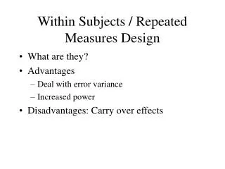
Advantages • Design – nonsystematic variance (i.e. error, that not under experimental control) is reduced • Take out variance due to individual differences • More sensitivity/power • Efficiency – fewer subjects are required
When to Use • Measuring performance on the same variable over time • for example looking at changes in performance during training or before and after a specific treatment • The same subject is measured multiple times under different conditions • for example performance when taking Drug A and performance when taking Drug B • The same subjects provide measures/ratings on different characteristics • for example the desirability of red cars, green cars and blue cars • Note how we could do some RM as regular between subjects designs • Ex. Randomly assign to drug A or B
Independence in ANOVA • Analysis of variance as discussed previously assumes cells are independent • But here we have a case in which that is unlikely • For example, those subjects who perform best in one condition are likely to perform best in the other conditions
Partialling out dependence • Our differences of interest now reside within subjects and we are going to partial out differences between the subjects • This removes the dependence on subjects that causes the problem mentioned • For example: • Subject 1 scores 10 in condition A and 14 in condition B • Subject 2 scores 6 in condition A and 10 in condition B • In essence, what we want to consider is that both subjects score 2 less than their own overall mean score in condition A and 2 more than their own overall mean score in condition B
Partition of SS SStotal SSb/t subjects SSw/in subjects SStreatment SSerror
Partitioning the degrees of freedom kn-1 n-1 n(k-1) k-1 (n-1)(k-1)
Sources of Variance • SStotal • Deviation of each individual score from the grand mean • SSb/t subjects • Deviation of subjects' individual means (across treatments) from the grand mean. • In the RM setting, this is largely uninteresting, as we can pretty much assume that ‘subjects differ’ • SSw/in subjects: How Ss vary about their own mean, breaks down into: • SStreatment • As in between subjects ANOVA, is the comparison of treatment means to each other (by examining their deviations from the grand mean) • However this is now a partition of the within subjects variation • SSerror • Variability of individuals’ scores about their treatment mean
Example • Effectiveness of mind control for different drugs
Calculating SS • Calculate SSwithin • Conceptually: • Reflects the subjects’ scores variation about their own individual means • (3-5)2 + (4-5)2… (4-2)2 + (3-2)2 = 58 • This is what will be broken down into treatment and error variance
Calculating SS • Calculate SStreat • Conceptually it is the sum of the variability due to all treatment pairs • If we had only two treatments, the F for this would equal t2 for a paired samples t-test • SStreat = • SStreat = • SStreat = 5[(1-3)2 + (2-3)2 + (4-3)2 + (5-3)2] = 50 5 people in each treatment Treatment means Grand mean
Calculating SS • SSerror • Residual variability • Unexplained variance, which includes subject by treatment interaction* • Recall that SSw/in = SStreat + SSerror • SSerror = SSw/in - SStreat • 58-50= 8
SPSS output • PES = 50/58 • Note that as we have partialled out error due to subject differences, our measure of effect here is • SSeffect/(SSeffect+ SSerror) • So this is PES not simply eta2 as it was for one-way between subjects ANOVA
Interpretation • As with a regular one-way Anova, the omnibus RM analysis tells us that there is some difference among the treatments (drugs) • Often this is not a very interesting outcome, or at least, not where we want to stop in our analysis • In this example we might want to know which drugs are better than which
Contrasts and Multiple Comparisons • If you had some particular relationship in mind you want to test due to theoretical reasons (e.g. a linear trend over time) one could test that by doing contrast analyses (e.g. available in the contrast option in SPSS before clicking ok). • This table compares standard contrasts available in statistical packages • Deviation, simple, difference, Helmert, repeated, and polynomial.
Multiple comparisons • With our drug example we are not dealing with a time based model and may not have any preconceived notions of what to expect • So now how are you going to do conduct a post hoc analysis? • Technically you could flip your data so that treatments are in the rows with their corresponding score, run a regular one-way ANOVA, and do Tukey’s etc. as part of your analysis. • However you would still have problems because the appropriate error term would not be used in the analysis. • B/t subjects effects not removed from error term
Multiple comparisons • The process for doing basic comparisons remains the same • In the case of repeated measures, as Howell notes (citing Maxwell) one may elect in this case to test them separately as opposed to using a pooled error term* • The reason for doing so is that such tests would be extremely sensitive to departures from the sphericity assumption • However using the MSerror we can test multiple comparisons (via programming) and once you have your resulting t-statistic, one can get the probability associated with that
Example in R comparing placebo and Drug A • t = 1.93 • pt(1.93, 4, lower.tail=F) • .063 one-tailed or .126 two-tailed MSerror from ANOVA table
Multiple comparisons • While one could correct in Bonferroni fashion, there is a False discovery rate for dependent tests • Will control for overall type I error rate among the rejected tests • The following example uses just the output from standard pairwise ts for simplicity
Multiple comparisons • Output from t-tests
Multiple comparisons • Output from R • The last column is the Benjamini and Yekutieli correction of the p-value that takes into account the dependent nature of our variables • A general explanation might lump Drug A as ineffective (not statistically different from the placebo), and B & C similarly effective
Assumptions • Standard ANOVA assumptions • Homogeneity of variances • Normality • Independent observations • For RM design we are looking for homogeneity of covariances among the treatments e.g. t1,t2,t3 • Special case of HoV • Spherecity • When the variance of the difference scores for any pair of groups is the same as for any other pair
Sphericity • Observations may covary across time, dose etc., and we would expect them to. But the degree of covariance must be similar. • If covariances are heterogeneous, the error term will generally be an underestimate and F tests will be positively biased • Such circumstances may arise due to carry-over effects, practice effects, fatigue and sensitization
Sphericity • Suppose the repeated measure factor of TIME had 3 levels – before, after and follow-up scores for each individual • RM ANOVA assumes that the 3 correlations • r ( Before-After ) • r ( Before-Follow up ) • r ( After-Follow up ) • Are all about the same in size • i.e. any difference due to sampling error
Sphericity • If they are not, then tests can be run to show this the Mauchly test of Sphericity generates a significant chi square • Again, when testing assumptions we typically hope they do not return a significant result • A correction factor called EPSILON is applied to the degrees of freedom of the error term when calculating the significance of F. • This is default output for some statistical programs
Sphericity • If the Mauchly Sphericity test is significant, then use the Corrected significance value for F • Otherwise use the “Sphericity Assumed” value • If there are only 2 levels of the factor, sphericity is not a problem since there is only one correlation/covariance.
Correcting for deviations • Epsilon ( measures the degree to which covariance matrix deviates from compound symmetry • All the variances of the treatments are equal and covariances of treatments are equal • When = 1 then matrix is symmetrical, and normal df apply • When = then matrix has maximum heterogeneity of variance and the F ratio should have 1, n-1 df
Estimating F • Two different approaches, adjusting the df • Note that the F statistic will be the same, but the df will vary • Conservative: Box's/Greenhouse-Geisser • Liberal: Huynh-Feldt • Huynh-Feldt tends to overestimate (can be > 1, at which point it is set to 1) • Some debate, but Huynh-Feldt is probably regarded as the method of choice, see Glass & Hopkins
Another RM example • Students were asked to rate their stress on a 50 point scale in the week before, the week of, or the week after their midterm exam
Data • Data obtained were:
Analysis • For comparison, first analyze these data as if they were from a between subjects design • Then conduct the analysis again as if they come from a repeated measures design
SPSS • “Analyze” “General Linear Model” “Repeated Measures” • Type “time” into the within-subject factor name text box (in place of “factor1”) • Type “3” in the Number of Levels box • Click “Add” • Click “Define”
Move the variables related to the treatment to the within subjects box • Select other options as desired
+ Comparing outputs • Between-subjects • Within subjects
Comparing outputs • SS due to subjects has been discarded from the error term in the analysis of the treatment in the RM design • Same b/t treatment effect • Less in error term • More power in analyzing as repeated measures
Another example (from Howell) • An experiment designed to look at the effects of a relaxation technique on migraine headaches • 9 subjects are asked to record the number of hours of such headaches each week to provide a baseline, then are given several weeks of training in relaxation technique – during which the number of hours of migraines per week were also recorded • A single within-subject effect with 5 levels (week 1, week 2, week 3, week 4, week 5)
Results • Summary table Note however that we really had 2 within subjects variables condition (baseline vs. training) and time (week 1-5) How would we analyze that? Tune in next week! Same bat time! Same bat channel!
Review - Covariance • Measure the joint variance of two (or more) variables • Use cross product of deviation of scores from their group mean • Formula: