CSS 650 Advanced Plant Breeding
CSS 650 Advanced Plant Breeding. Module 1: Introduction Population Genetics Hardy Weinberg Equilibrium Linkage Disequilibrium. Plant Breeding. “The science, art, and business of improving plants for human benefit” Considerations: Crop(s) Production practices End-use(s)

CSS 650 Advanced Plant Breeding
E N D
Presentation Transcript
CSS 650 Advanced Plant Breeding Module 1: Introduction Population Genetics Hardy Weinberg Equilibrium Linkage Disequilibrium
Plant Breeding “The science, art, and business of improving plants for human benefit” Considerations: • Crop(s) • Production practices • End-use(s) • Target environments • Type of cultivar(s) • Traits to improve • Breeding methods • Source germplasm • Time frame • Varietal release and intellectual property rights Bernardo, Chapter 1
Plant Breeding A common mistake that breeders make is to improve productivity without sufficient regard for other characteristics that are important to producers, processors and consumers. • Well-defined Objectives • Good Parents • Genetic Variation • Good Breeding Methods • Functional Seed System • Adoption of Cultivars by Farmers
Quantitative Traits • Continuum of phenotypes (metric traits) • Often many genes with small effects • Environmental influence is greater than for qualitative traits • Specific genes and their mode of inheritance may be unknown • Analysis of quantitative traits • population parameters • means • variances • molecular markers linked to QTL
Populations • In the genetic sense, a population is a breeding group • individuals with different genetic constitutions • sharing time and space • In animals, mating occurs between individuals • ‘Mendelian population’ • genes are transmitted from one generation to the next • In plants, there are additional ways for a population to survive • self-fertilization • vegetative propagation • Definition of ‘population’ may be slightly broader for plants • e.g., lines from a germplasm collection Falconer, Chapt. 1; Lynch and Walsh, Chapt. 4
What do population geneticists do? Study genes in populations • Frequency and interaction of alleles • Mating patterns, genotype frequencies • Gene flow • Selection and adaptation vs random genetic drift • Genetic diversity and relationship • Population structure Related Fields • Evolutionary Biology – e.g., crop domestication • Landscape Genetics
Gene and genotype frequencies p + q = 1 For a population of diploid organisms: P11 + P12 + P22 = 1 Bernardo, Chapter 2
Gene frequencies (another way) Number of individuals = N = N11+ N12+ N22 = 100 Number of alleles = 2N = N1 + N2 = 200
Inbred x inbred Alleles are unknown, but allele frequencies at segregating loci are known F1 and F2: p = q = 0.5 Allele frequencies in crosses Value of q is reduced by ½ in each backcross generation
Factors that may change gene frequencies • Population size • changes may occur due to sampling • assume ‘large’ population • Differences in fertility and viability • parents may differ in fertility • gametes may differ in viability • progeny may differ in survival rate • assume no selection • Migration and mutation • assume no migration and no mutation
Factors that may change genotype frequencies Changes in genotype frequency (not gene frequency) • Mating system • assortative or disassortative mating • selfing • geographic isolation • assume that mating occurs at random (panmixia)
Hardy-Weinberg Equilibrium • Assumptions • large, random-mating population • no selection, mutation, migration • normal segregation • equal gene frequencies in males and females • no overlap of generations (no age structure) • Note that assumptions only need to be true for the locus in question • Gene and genotype frequencies remain constant from one generation to the next • Genotype frequencies in progeny can be predicted from gene frequencies of the parents • Equilibrium attained after one generation of random mating
Hardy-Weinberg Equilibrium A1 A2 A1 p2=.16 pq=.24 p = 0.4 A2 q = 0.6 Expected genotype frequencies are obtained by expanding the binomial (p + q)2 = p2 + 2pq + q2 = 1 q2=.36 pq=.24
Equilibrium with multiple alleles For multiple alleles, expected genotype frequencies can be found by expanding the multinomial (p1 + p2 + ….+ pn)2 For example, for three alleles: Corresponding genotypes: A1A1 A1A2 A1A3 A2A2 A2A3 A3A3 Lynch and Walsh (pg 57) describe equilibrium for autopolyploids
A1A1 A2A2 A1A2 Relationship between gene and genotype frequencies • f(A1A2) has a maximum of 0.5, which occurs when p=q=0.5 • Most rare alleles occur in heterozygotes • Implications for • F1? • F2? • Any BC?
Applications of the Hardy-Weinberg Law • Predict genotype frequencies in random-mating populations • Use frequency of recessive genotypes to estimate the frequency of a recessive allele in a population • Example: assume that the incidence of individuals homozygous for a recessive allele is about 1/11,000. q2 = 1/11,000q 0.0095 • Estimate frequency of individuals that are carriers for a recessive allele p = 1 - 0.0095 = 0.9905 2pq = 0.0188 2%
Testing for Hardy-Weinberg Equilibrium All genotypes must be distinguishable N = N11+ N12+ N22= 233 + 385 + 129 = 747
Chi-square test for Hardy-Weinberg Equilibrium • Accept H0: no reason to think that assumptions for Hardy-Weinberg equilibrium have been violated • does not tell you anything about the fertility of the parents • When you reject H0, there is an indication that one or more of the assumptions is not valid • does not tell you which assumption is not valid Example in Excel only 1 df because gene frequencies are estimated from the progeny data
Exact Test for Hardy-Weinberg Equilibrium • Chi-square is only appropriate for large sample sizes • If sample sizes are small or some alleles are rare, Fisher’s Exact test is a better alternative • Calculate the probability of all possible arrays of genotypes for the observed numbers of alleles • Rank outcomes in order of increasing probability • Reject those that constitute a cumulative probability of <5% Example in Excel Weir (1996) Chapt. 3
Likelihood Ratio Test Maximum of the likelihood function given the data (z) when some parameters are assigned hypothesized values Maximum of the likelihood function given the data (z) when there are no restrictions When the hypothesis is true: 2 df=#parameters assigned values Likelihood ratio tests for multinomial proportions are often called G-tests (for goodness of fit) Lynch and Walsh Appendix 4
Likelihood Ratio Test for HWE where is the expected number and is the observed number of the ijth genotype Calculations in Excel
B b PAB PAb pA A a PaB Pab pa pB pb B b A .40 .10 .50 a .10 .40 .50 .50 .50 Gametic phase equilibrium Random association of alleles at different loci (independence) PAB=pApB Disequilibrium DAB = PAB – pApB DAB = PABPab – PAbPaB DAB = 0.40 – 0.5*0.5 = 0.15 DAB = 0.4*0.4 – 0.1*0.1 = 0.15 Lynch and Walsh, pg 94-100; Falconer, pg 15-19
Linkage Disequilibrium • Nonrandom association of alleles at different loci • the covariance in frequencies of alleles between the loci • Refers to frequencies of alleles in gametes (haplotypes) • May be due to various causes in addition to linkage • ‘gametic phase disequilibrium’ is a more accurate term • ‘linkage disequilibrium’ (LD) is widely used to describe associations of alleles in the same or in different linkage groups
Linkage Disequilibrium Excess of coupling phase gametes +D Excess of repulsion phase gametes -D
Sources of linkage disequilibrium • Linkage • Multilocus selection (particularly with epistasis) • Assortative mating • Random drift in small populations • Bottlenecks in population size • Migration or admixtures of different populations • Founder effects • Mutation
A A B B A b a b 0.5 AB 0.5 Ab 0.25 AB 0.25 aB 0.25 Ab 0.25 ab Two locus equilibrium • For two loci, it may take many generations to reach equilibrium even when there is independent assortment and all other conditions for equilibrium are met • New gamete types can only be produced when the parent is a double heterozygote
Decay of linkage disequilibrium • In the absence of linkage, LD decays by one-half with each generation of random mating c = recombination frequency
Factors that delay approach to equilibrium • Linkage • Selfing – because it decreases the frequency of double heterozygotes • Small population size – because it reduces the likelihood of obtaining rare recombinants
Implications for breeding • Gametic Phase Disequilibrium that is not due to linkage is eliminated by making the F1 cross • Recombination occurs during selfing • There would be greater recombination with additional random mating, but it may not be worth the time and resources P1P2 A1A1B1B1 x A2A2B2B2 F1 A1A2B1B2 gametefrequency A1B1 0.5*(1-c) A1B2 0.5*c A2B1 0.5*c A2B2 0.5*(1-c)
no linkage Effect of mating system on LD decay c = effective recombination rate s = the fraction of selfing 99% selfing outcrossing
Alternative measures of LD fyi • D is the covariance between alleles at different loci • Maximum values of D depend on allele frequencies • It is convenient to consider r2 to be the square of the correlation coefficient, but it can only obtain a value of 1 when allele frequences at the two loci are the same • r2indicates the degree of association between alleles at different loci due to various causes (linkage, mutation, migration)
D – minimum and maximum values If D>0 Look for the maximum value D can have PAb = pApb - D 0 D pApb PaB = papB - D 0 D papB D min(pApb, papB) If D<0 Look for the minimum value D can have PAB = pApB + D 0 D -pApB Pab = papb + D 0 D -papb D max(-pApB, -papb)
Alternative measures of LD fyi • D’ is scaled to have a minimum of 0 and a maximum of 1 • D’ indicates the degree to which gametes exhibit the maximum potential disequilbrium for a given array of allele frequencies • D’=1 indicates that one of the haplotypes is missing • D’ is very unstable for small sample sizes, so r2 is more widely utilized to measure LD When DAB > 0 When DAB < 0
Testing for gametic phase disequilibrium • Best when you can determine haplotypes • inbred lines or doubled haploids • haplotypes of double heterozygotes inferred from progeny tests • Use a Goodness of Fit test if the sample size is large • Chi-square • G-test (likelihood ratio) • Use Fisher’s exact test for smaller sample sizes • Use a permutation test for multiple alleles • Need a fairly large sample to have reasonable power for LD (~200 individuals or more) See Weir (1996) pg 112-133 for more information
Depiction of Linkage Disequilibrium Disequilibrium matrix for polymorphic sites within sh1 in maize Prob valueFisher’s Exact Test r2 Flint-Garcia et al., 2003. Annual Review of Plant Biology 54: 357-374.
Extent of LD in Maize Average LD decay distance is 5–10 kb r2 Linkage disequillibrium across the 10 maize chromosomes measured with 914 SNPs in a global collection of 632 maize inbred lines. Yanet al. 2009. PLoS ONE 4(12): e8451
Extent of LD in Barley Elite North American Barley No adjustment for population structure Average LD decay distance is ~5 cM r2 Adjusted for population structure • Other studies • Wild barley – LD decays within a gene • Landraces ~ 90 kb • European germplasm - significant LD: • mean 3.9 cM, median 1.16 cM Waugh et al., 2009, Current Opinion in Plant Biology 12:218-222
References on linkage disequilibrium Flint-Garcia et al., 2003. Structure of linkage disequilibrium in plants. Annual Review of Plant Biology 54: 357-374. Gupta et al., 2005. Linkage disequilibrium and association studies in higher plants: present status and future prospects. Plant Molecular Biology 57:461–485. Slatkin, M. 2008. Linkage disequilibrium – understanding the evolutionary past and mapping the medical future. Nature Reviews Genetics 9:477–485 Waugh, R., Jean-Luc Jannink, G.J. Muehlbauer, L. Ramsay. 2009. The emergence of whole genome association scans in barley. Current Opinion in Plant Biology 12(2): 218–222. Yan, J., T. Shah, M.L Warburton, E.S. Buckler, M.D. McMullen, et al. 2009. Genetic characterization and linkage disequilibrium estimation of a global maize collection using SNP Markers. PLoS ONE 4(12): e8451. Zhu et al., 2008. Status and prospects of association mapping in plants. The Plant Genome 1: 5–20.