Integration
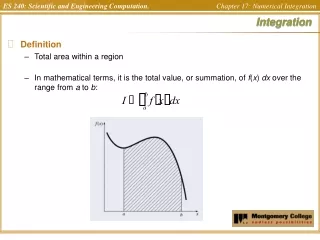
Integration. Definition Total area within a region In mathematical terms, it is the total value, or summation, of f ( x ) dx over the range from a to b :. Newton-Cotes Formulas. General Idea replace a complicated function or tabulated data with a polynomial that is easy to integrate:

Integration
E N D
Presentation Transcript
Integration • Definition • Total area within a region • In mathematical terms, it is the total value, or summation, of f(x) dx over the range from a to b:
Newton-Cotes Formulas • General Idea • replace a complicated function or tabulated data with a polynomial that is easy to integrate: • where fn(x) is an nth order interpolating polynomial.
Newton-Cotes Illustrations • The integrating function can be polynomials for any order - for example, (a) straight lines or (b) parabolas. • The integral can be approximated in one step or in a series of steps to improve accuracy.
The Trapezoidal Rule • Uses straight-line approximation for the function • Uses linear interpolation
Error of the Trapezoidal Rule • The error is dependent upon the curvature of the actual function as well as the distance between the points. • Error can thus be reduced by: • breaking the curve into parts or • using a higher order function
Composite Trapezoidal Rule • Assuming n+1 data points are evenly spaced, there will be n intervals over which to integrate. • The total integral can be calculated by integrating each subinterval and then adding them together:
Trapezoid Functions • For inline functions, use the ‘trap functions • For tabulated data, use trapz(x,y) • Matlab built-in function for numerical integration based on trapezoidal rule • y(x) should be in a tabulated form • can handle unequally spaced data as long as x in ascending order • example: >> x=[0 .12 .22 .32 .4 .44 .54 .64 .7 .8]; >> y=0.2+25*x-200*x.^2+675*x.^3-900*x.^4+400*x.^5; >> trapz(x,y) 1.5948
Trapezoid Rule Examples • Tabulated • Inline Function % f(x)=cos(x)+sin(2x) on [0 pi/2] h=(pi/2-0)/10; >> x=0:h:pi/2; >> y=cos(x)+sin(2*x); >> I2=trapz(x,y) 1.9897 p=inline('cos(x)+sin(2*x)'); >> I3=trap(p,0,pi/2,10) 1.9897 % plot f(x) and I(x) >> for k=1:11 I4(k)=trap(p,0,x(k),20); end; >> plot(x,y,x,I4,'r')
Simpson’s Rules • Increasing the approximation order results in better integration accuracy • Simpson’s 1/3 rule • based on taking 2nd order polynomial integrations • use two panels (three points) every integral • only for even number of panels • Simpson’s 3/8 rule is • based on taking 3rd order polynomial integrations • use three panels (four points) every integral • only for three-multiple number of panels
Simpson’s 1/3 Rule • Using the Lagrange form for a quadratic fit of three points: • Integration over the three points simplifies to: • Composite
Simpson’s 3/8 Rule • Basic • Composite
Combined Simpson’s Rule • Combined Simpson’s rule • If n (number of panels) is even, use Simpson’s 1/3 rule • If n is odd, use Simpson’s 3/8 rule once at beginning or end and use Simpson’s 1/3 rule for the rest of the panels
Error of Simpson’s 1/3 Rule • If f(x) is a polynomial function of degree 3 or less, Simpson’s rule provides no error. • Use smaller spacing (h decreases) or more panels to reduce the error. • In general, Simpson’s rule is accurate enough for the most of functions f(x) with much less panels compared to that with the trapezoidal rule.
Simpson’s Rule Example • By Hand • Fucntions x=[0.1 0.2 0.3 0.4 0.5 0.6 0.7]; y=[2.1 1.7 1.6 2.3 2.8 1.7 2.5]; 0=(0.1/3)*(y(1)+4*y(2)+2*y(3)+ 4*y(4)+2*y(5)+4*y(6)+y(7)) >>1.2067 % f(x)=cos(x)+sin(2x) on [0 pi/2] n=10; h=(pi/2-0)/10; % 10panels x=0:h:pi/2; y=cos(x)+sin(2*x); I2=0; for k=1:2:(n-1) I2=I2+h/3*(y(k)+4*y(k+1)+y(k+2)); end 2.0001 • % define function f(x) • p=inline('cos(x)+sin(2.*x)'); • I3=simps(p,0,pi/2,10) • 2.0001 • Try different number of panels • Compare with trapezoid rule
Lab • Ex 17.3