
SlideServe
Menu
Préférences
© SlideServe · v2026

Introduction to Numerical Integration: Trapezoidal and Simpson’s Rules Explained

nemesio-lazaro avatar
11 diapositives · 364 Views · Nov 20, 2014

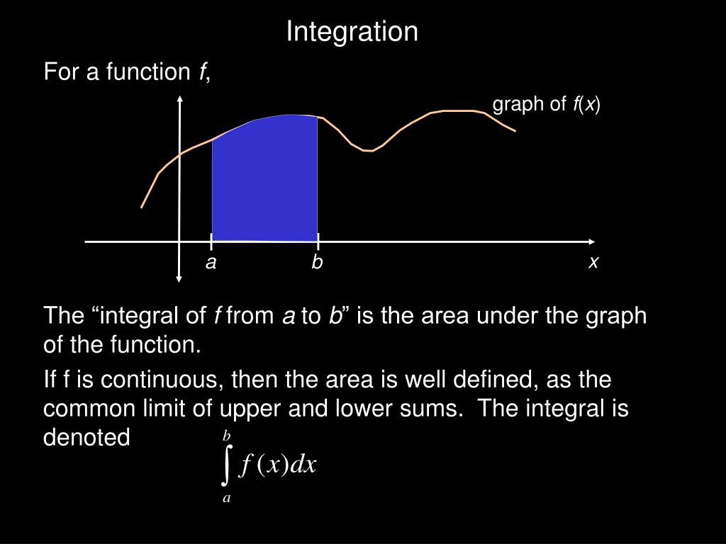
This document provides a comprehensive overview of numerical integration techniques, focusing on the Trapezoidal and Simpson's rules. It begins with the definition of the integral of a function ( f ) as the area under its graph between points ( a ) and ( b ). The Trapezoidal rule is illustrated through composite approximations, and key concepts are presented for evaluating integrals using Simpson’s Rule for a cubic polynomial. Additionally, adaptive step size methods and stopping criteria for numerical integration are discussed, enhancing the accuracy of numerical estimates.
Introduction to Numerical Integration: Trapezoidal and Simpson’s Rules Explained - slide 1
01 / 11Introduction to Numerical Integration: Trapezoidal and Simpson’s Rules Explained
1 / 17

Télécharger la présentation

Introduction to Numerical Integration: Trapezoidal and Simpson’s Rules Explained
Une image / un lien ci-dessous est fourni (tel quel) pour télécharger la présentation

Politique de téléchargement : le contenu du site vous est fourni TEL QUEL pour votre information et votre usage personnel ; il ne peut être vendu, concédé sous licence ni partagé sur d’autres sites sans l’accord de son auteur.Le contenu vous est fourni TEL QUEL, pour votre information et votre usage personnel uniquement. Téléchargez la présentation en cliquant sur ce lien. Lors du téléchargement, si vous ne parvenez pas à télécharger une présentation, l’éditeur a peut-être supprimé le fichier de son serveur.Pendant le téléchargement, si vous ne parvenez pas à obtenir une présentation, le fichier a peut-être été supprimé par l’éditeur.

F I N

Plus de contenu associé

Transcription de la présentation
  1. Integration For a function f, The “integral of f from a to b” is the area under the graph of the function. If f is continuous, then the area is well defined, as the common limit of upper and lower sums. The integral is denoted graph of f(x) x a b

  2. Numerical Integration: Trapezoid graph of f(x) approximate this region x a b graph of f(x) with this trapezoid x a b

  3. Composite Trapezoid graph of f(x) Apply “trapezoid” approximation to k subdivisions of [a b] x a b graph of f(x) “trapezoid” approximation with 3 subdivisions of [a b] x a b

  4. Composite Trapezoid graph of f(x) “trapezoid” approximation with 3 subdivisions of [a b] x a b h Let h=(b-a)/3. The sum of all the approximations is

  5. Simpson’s Rule: Suppose f(x)=x Let a = 2 and b = 8 ½(64-4) = 30 1/6(6)(2 + 4*5 +8) = 30

  6. Derivation of Simpson’s Rule: Suppose f(x)=x3

  7. Simpson’s Rule: Derivation Put all of those together, along with Hence: If f is any cubic polynomial, then This is the basis for Simpson’s rule.

  8. Simpson’s Rule For any function f, the Simpson’s approximation to is and in the middle Evaluate the function at the endpoints

  9. Composite Simpson’s Rule graph of f(x) Simpson on 3 subdivisions of [a b] h=(b-a)/3 x a b h Add them up. Total of 7 function evaluations.

  10. Numerical Integration: Ad-Hoc stopping criteria Pick a method (trapezoid, or Simpson’s). Set a stopping tolerance TOL. Pick k, an initial number of subdivisions Iterate as below • Apply composite method using k divisions • Apply composite method using 2k divisions • If answers are within TOL, stop, and return the 2k division answer • If answers are not within TOL, increase k and repeat. .

  11. Adaptive Stepsize Only use small h (the “stepsize”) where the convergence demands it. Recursive implementation is straightforward. function I = adr(fh,a,b,tol) Compute I1 using 1 subdivision Compute I2 using 2 subdivisions If the answers are within tol, I = I2; Else m = (a+b)/2; ILeft = adr(fh,a,m,tol/2); IRight = adr(fh,m,b,tol/2); I = ILeft + IRight; end