CO 2 Source-Sink Matching
CO 2 Source-Sink Matching. Lunch Talk August 18, 2009 Weifeng Li. Introduction. CO 2 sources and geological sinks may be widely spatially dispersed and need to be connected through a CO 2 pipeline network.

CO 2 Source-Sink Matching
E N D
Presentation Transcript
CO2 Source-Sink Matching Lunch Talk August 18, 2009 Weifeng Li
Introduction • CO2 sources and geological sinks may be widely spatially dispersed and need to be connected through a CO2 pipeline network. • CO2 source-sink matching generates a fully integrated, optimal CCS network that minimizes the full mitigation cost for the network system subject to constraints of the sinks’ storage capacity.
Two-Step Approach • Identify candidate least-cost pipeline network between all sources and sinks • Optimize the source-sink allocation for a give set of CO2 sources and sinks that minimizes the full mitigation cost
Least-cost Pipeline Network • Pipeline construction costs vary considerably • Terrain • Crossings (waterways, railways, highways) • Protected areas • Populated areas • Obstacle layers (1x1km) are used to reverse-engineering the contribution (weight) of geographical features to the cost of pipeline construction. • MIT CO2 transport cost tool will identify the least-cost path and calculate its length for linking each source to sink.
Obstacle Conditions and Their Relative Cost Factors * Values are based on 8-inch diameter pipelines;
Assumptions • Pipeline path depends only on the geography feature of the obstacles; • The diameter (determined by mass flow rate) does not affect the pipeline path.
Potential pipeline routes (blue) between the 30 biggest CO2 sources (green) and 14 largest sinks.
Cost Overview Source: Economic Evaluation of CO2 Storage and Sink Enhancement Options (TVA Report to DOE) capture cost transport cost Injection cost
CO2 Capture Cost • Methodology • “Generic CO2 Capture Retrofit” spreadsheet prepared by SFA Pacific, Inc. • Three key input variables for the spreadsheet calculation • Flue gas flow rate (in metric tonnes per hour) • Flue gas composition (volume share or weight share of CO2 in flue gas) • Annual load factor
CO2 Capture Cost Source: SFC Pacific, Inc.
MIT Capture Cost Model: Assumptions • Capture efficiency • assumed to be 90% for non-pure CO2 sources, 100% for pure CO2 sources • CO2 quantity (flue gas flow rate) • Determined by design capacity • Operating factor (assumed to be 80% for power plants, 100% for non-power plants) • CO2 quality (flue gas composition) • Same for each fuel-type category(type of plant)
MIT Capture Cost Model: Assumptions Flue Gas Composition for Power Plants Note: Data about oil-fired power plants are MIT Carbon Capture and Sequestration Technologies Program estimates. Others are from SFA, Pacific "Generic CO2 Capture Retrofit“ and "Existing Coal Power Plant CO2 Migration“ spreadsheets.
CO2 Capture Cost Calculation • Nat Gas @ $5/MBtu • No Carbon Tax Coal-fired Power Plant
Capture Cost: Empirical Estimation X: design capacity Capture cost = ($/t CO2 captured) * flow rate
MIT CO2 Transport Cost Model • Module to calculate pipeline diameter (D) • Economic module to calculate the total and annualized CO2 pipeline transport cost
Pipeline Diameter Calculation: Methodology • the default maximum allowable pressure drop per unit length (∆P/∆L) is set to be 49Pa/m. • The default CO2 density (ρ) is assumed to be 884 kg/m3. • The Fanning friction pressure is found by using the relationship based on the Moody chart (see Heddle et.al., 2003).
Pipeline Diameter Calculation (X>1 Mt)
Pipeline Diameter Calculation – Implementation • Given a CO2 flow rate from the user and assuming a pressure drop of 49 Pa/m, we generated a look-up table for pipeline diameter.
Pipeline Diameter Calculation (X>1 Mt)
Pipeline Total Cost • General Equation • Annualized Cost = Land Construction Cost * Capital Charge Factor + O&M Cost • Capital Charge Factor • Use 0.15 by default • O&M Cost • The O&M cost is estimated to be $5,000*Length (in mile) per year, independent of pipeline diameter
Land Construction Cost (LCC) Calculation • MIT Correlation • LCC = a * D * L*Indext • a = $33,853; • D: pipeline diameter in inches (function of CO2 flow rate); • L: least-cost pipeline path length in miles; • Indext: optional extra for inflation (post 1998)
CO2 Injection Cost • Injectivity Model -> number of wells required • Cost Model -> total process cost
Injectivity Model Law & Bachu Method
Injection Cost Model • General Equation • Annualized Cost = Capital Cost * Capital Charge Factor + O&M Cost • Capital Charge Factor • Use 0.15 by default
Potential pipeline routes (blue) between the 30 biggest CO2 sources (green) and 14 largest sinks.
Scenarios • 2007 Transport Cost Base, assuming no EOR • 2007 Transport Cost Base, with EOR • MIT Transport Cost correlation, assuming no EOR • MIT Transport Cost correlation, with EOR
Pipeline network (blue) connecting 30 biggest CO2 sources (green) and largest sinks (EOR and oil/gas fields, aquifers).
2007 Cost base: no EOR 2007 Cost base: with EOR MIT cost correlation: no EOR MIT cost correlation : with EOR
2007 Cost base: no EOR 2007 Cost base: with EOR MIT cost correlation: no EOR MIT cost correlation : with EOR
Thank You! Questions?