2.2a Aggregate Demand

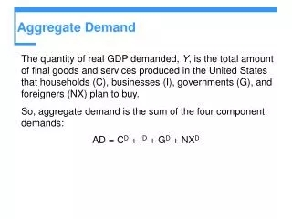
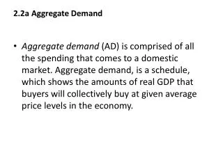
1. 2.2a Aggregate Demand • Aggregate demand (AD) is comprised of all the spending that comes to a domestic market. Aggregate demand, is a schedule, which shows the amounts of real GDP that buyers will collectively buy at given average price levels in the economy.

2. Therefore we categorize the different types of demand like this: • Consumer spending (C) • Investment (I) • Government spending (G) • Net Exports (X – M)

3. The aggregate demand curve has a negative slope. Essentially the AD curve is the visual representation of the expenditure method of GDP accounting. • The price level is measured as the average price level of final goods and services (product) in the economy and is considered a measurement of inflation.

4. Why is the AD curve negatively sloped? • The first reason is called the real balances effect. As the price level rises, the purchasing power of the public’s income or savings decreases so they can buy less as the price level rises. This factor is most closely associated with consumption (C).

5. Secondly, the interest rate effect influences the slope. As prices rise, there is an increase in demand for money and the cost of borrowing money (the interest rate) will rise as well. Lenders will charge a higher rate of interest for the public to borrow money to finance household consumption or for firms to invest in productive capacity. This effect is usually most visible in investment (I).

6. Finally there is the foreign purchases effect. When the price level rises, it makes the country’s exports more expensive to foreign buyers. This leads to a decrease in foreign purchases of the country’s exports. Moreover, rising domestic prices may make imported goods cheaper and result in citizens substituting imports for exports at higher price levels. This is effect is seen in net exports (X – M).

8. In the diagram above, the economy is producing output Y at the price level P. • Shifts in the AD curve are the result of changes in the components of AD or changes in the factors of the following equation: C + I +G + (X – M) = AD

9. Consumption – The elements that affect consumer spending would be changes in the following: Consumer wealth – While changes in income will clearly change consumption, so will the wealth of households. If there is a change in the value of physical (real estate) or paper (stocks and bonds) assets, then consumers will feel more or less wealthy and adjust their spending accordingly.

10. Consumer expectations – If consumers believe that their real income will change in the future, they will increase or reduce expenditures based upon their expectations. • Personal income taxes – A direct tax will affect disposable income which will have an impact upon households ability to consume.

11. Household indebtedness – When households borrow to consume (or invest), the purchases bought with borrowed money will increase AD. However, when consumers pay back that debt, they will have to reduce current expenditures to pay back for previous consumption which will decrease AD.

12. Interest rates – The cost of borrowing money will impact the purchase of “big ticket” items or consumer durable goods. These are goods that last longer than a year and are difficult for households to buy without borrowing moneyIf interest rates are low, then households would be willing to borrow money to buy the goods they desire, thereby increasing AD as noted above.

13. Investment spending – Investment is the most volatile variable in AD because it relies upon future expectations of businesses and individuals of economic activity. The elements that affect business investment would be changes in the following:

14. Real interest rates – Again, the cost of borrowing money can induce businesses to take or put off investing. If the real interest rate increases, then businesses will hold off borrowing to buy new plant and equipment. If real interest rates decrease, then firms would increase investment with a corresponding increase in AD.

15. Expected returns – If companies believe that they will be able to make a good return on investment, then they will increase their purchases and shift the AD curve to the right. If businesses believe that business conditions will improve, then they will invest in new projects.

16. Business taxes – Taxes will have a direct effect upon the profits that a firm expects to make from an investment. Consequently, a reduction in business taxes will increase investment and AD. An increase in such taxes will have the opposite effect.

17. Technology – Improvements in technology, which bring with them a corresponding increase in productivity, will increase returns to an investment. Technological change incentivizes firms to increase their investment, which then leads to an increase in AD.

18. Government spending – The elements that affect government spending would be changes in the following: Changes in political priorities – If a government decides to change spending due to a perceived threat or crisis then the G variable will impact AD. An example might be a change in defense expenditures.

19. Changes in economic priorities – In the case of a recessionary environment, the government may increase expenditures to make up for the loss of AD or employment that occurs in a downturn. An example of this might be increasing expenditures on infrastructure such as roads.

20. Net Export spending would be affected by the following: National income abroad – When trade partners incomes rise, they have a tendency to buy more imports, which could mean an increase in purchases of our exports. The opposite is true if their incomes decrease.

21. Exchange rates – When our country’s currency depreciates, it makes our exports cheaper to foreign buyers as it takes fewer units of their currency to pay for the goods or services we sell them. This will increase AD. Conversely, we may see the opposite effect if our currency appreciates against that of our trade partners.

22. Levels of protectionism – If there is increased protectionism (import tariffs or quotas) practiced by trade partners, this can reduce exports and thereby AD.

23. 2.2b Aggregate supply • Aggregate supply (AS) is a schedule of real domestic output that is produced at each possible price level. • Unlike aggregate demand, aggregate supply is more complex in its measurement. This is due to the fact that producers cannot adjust quickly to changes in the average price level.

24. The short run is defined as the timeframe in which wages and input prices cannot adjust to changes in the average price level. • The long run is considered to be the time in which wages and input prices can adjust to changes in the average price level.

25. Movements along the SRAS curve – • Due to what we call a recognition lag, wages and factor input costs do not respond immediately to changes in the price level so it takes time for these prices to adjust. • While an increase in the price level might allow a firm to increase its product prices, the factor input costs will respond much more slowly.

26. Remember that the largest cost for most firms is labor and so the nominal wage rate plays a dominant role in firms’ operations. • Wage rate changes often lag changes in the price level in an economy as it takes time for workers to realize that their purchasing power has declined. • When the price level rises, firms are able to increase their final goods prices and make larger profits as their wage bill remains unchanged.

27. Subsequently, a firm will increase its output when the price level is rising to capture more profits. • Consequently, the firms increase output and can push the economy beyond full employment as they hire unemployed workers and encourage employees to work overtime or to move to full time work.

28. The situation is illustrated in the diagram below at point b in which the Y’ level of RGDP at the P’ price level demonstrates a rise up along the SRAS curve.

29. Firms respond to falls in the price level by lowering their final goods prices as they attempt to clear inventory. • This reduction in sales revenues will reduce profits and put firms in a position to decrease production or even lay off workers. The increase in unemployment will correspond to a decrease in SRAS. • This condition corresponds to the Y” level of RGDP at the P” price level or at point c on the diagram below.

30. The movements along the SRAS curve described above originate at point a.

31. Production costs are the primary factor in changes in AS. However, there are several determinants of AS:

32. Resource costs – All factor input prices will play a role in the final product price, consequently any change in resource costs will shift the curve. If for example, there is a decrease in the price of oil, then the AS curve will shift out to the right as we can produce more output with the same expenditure as before the price change. Conversely, a rise in wages will push the curve up and to the left.

33. Resource costs are not just domestic in nature. While labor is a domestic expense, some raw materials are imported. As a result, exchange rates and control over the supply of the needed resource can complicate prices firms.

34. If one particular trade partner has inordinate market power over a commodity, then it can increase the price and thereby impact our AS due to our use of the input in our production. Furthermore, if our exchange rate depreciates, we will have to pay more for imports of a critical factor input.

35. Productivity – Improvements in productivity will increase output at all price levels and push the AS out and to the right. • By improving the quality of factor inputs, either in the case of new machines or increasing the skill level of workers, we can produce more output at current prices and shift out the AS curve.

36. Business Environment – This addresses many variables such as: • Business taxes – Higher direct and indirect taxes increase costs in the short run and can lead to a reduction in output at every price level with a corresponding leftward shift in the AS curve.

37. Subsidies – Payments by the government to firms to encourage the production of specific goods can lower production costs and encourage companies to expand their output. • Regulation - The costs associated with complying with government regulations can divert funds from production and decrease output for firms. An increase in government regulation may shift the AS curve to the left.

38. 2.2c Controversy over aggregate supply Aggregate supply is a source ofdebate among different schools of economic thought. Most economists agree that the long run AS (LRAS) curve is vertical and that it represents the full employment/potential level of output.

39. Neo- Classical economists (Friedrich Hayek and Milton Friedman) argue thatproduction levels are determined through the efficient operation of markets. Therefore, there is no SRAS as the economy is always just at full employment operating on or near the LRAS curve.

40. If there is a temporary downturn, then laid off workers will quickly adjust their wage demands or change their location and be reemployed very soon. There is no need for the government to intervene • Neo-classical economists believe that any policy to address instability in the economy will interfere with the self-correcting mechanism of markets and result in price distortions (inflation).

41. In essence, the neo-classical perspective believes that AS in the long run is independent of prices as markets will act to push the economy back towards equilibrium.

42. The neo-classical school is often associated with non-interventionist and market based policies. By reducing the role of government in the economy and regulating the rate of growth in the money supply (more on this later), markets will self-correct and the economy will grow more effectively.

43. Consequently, neo-classical economists focus on the long run and as a result they will push for supply-side policies which reduce impediments to competition as well as reduce government intervention in the economy.

44. Neo-classical attitudes are connected to mostly right leaning political parties. Policies promoted in Ireland in the period after the 2009 financial crisis which reduced government spending and encouraged austerity in general, could be considered to be neo-classical in nature.

45. However, Keynesian economists believe that markets are imperfect and that macroeconomic instability is the result of different forms of market failure. • Consequently, the Keynesians believe in the AS curve which has three regions.

46. They believe that output can fall at such as rate that it falls into the horizontal range of the AS curve. This means that there could be a decrease in output with no change in the price level. • This is due to the belief that resource costs and final product prices are “sticky downwards”. This perspective is rooted in the belief that workers do not adjust their wage demands as rapidly as they will attempt to find employment at their previous income.

47. Moreover, from this perspective, producers do not adjust their product prices until absolutely necessary to clear inventory. • When both of these scenarios are in play, there is plenty of spare capacity for the economy to put back to work without putting upward pressure on the price level.

48. Horizontal range – this is substantially below full employment implies that the economy is in recession or worse, a depression. There are plenty of unemployed resources and there is upward pressure on prices. This is characterized by a flat portion of the AS curve.

49. Intermediate range – as the economy starts to grow, there is increased demand for labor and other resources. This results in upward pressure on factor input prices and requires firms to increase their product prices to maintain profitability. There will begin to be shortages of resources, which will further drive up prices. This region is where most of the short run analysis is done and is upward sloping.

50. Vertical range – when the economy reaches its potential output or full employment, the curve becomes vertical. This is because the economy is at full capacity. Any efforts by firms to increase output will only bid resources away from other firms and drive up prices in the process. This is due to the finite resources in the economy.