Optimization with Lagrangian Multiplier Method in Constrained Maximization
Learn about the Lagrangian multiplier method for solving constrained optimization problems, maximizing functions subject to constraints, and the economic interpretations of the Lagrange multiplier in cost-benefit analysis.

Optimization with Lagrangian Multiplier Method in Constrained Maximization
E N D
Presentation Transcript
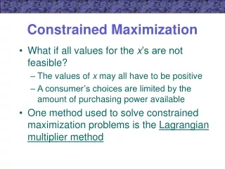
Constrained Maximization • What if all values for the x’s are not feasible? • The values of x may all have to be positive • A consumer’s choices are limited by the amount of purchasing power available • One method used to solve constrained maximization problems is the Lagrangian multiplier method
Lagrangian Multiplier Method • Suppose that we wish to find the values of x1, x2,…, xn that maximize y = f(x1, x2,…, xn) subject to a constraint that permits only certain values of the x’s to be used g(x1, x2,…, xn) = 0
Lagrangian Multiplier Method • The Lagrangian multiplier method starts with setting up the expression L = f(x1, x2,…, xn ) + g(x1, x2,…, xn) where is an additional variable called a Lagrangian multiplier • When the constraint holds, L = f because g(x1, x2,…, xn) = 0
. . . L/xn = fn + gn = 0 Lagrangian Multiplier Method • First-Order Conditions L/x1 = f1 + g1 = 0 L/x2 = f2 + g2 = 0 L/ = g(x1, x2,…, xn) = 0
Lagrangian Multiplier Method • The first-order conditions can be solved for x1, x2,…, xn and • The solution will have two properties: • The x’s will obey the constraint • These x’s will make the value of L (and therefore f) as large as possible
Lagrangian Multiplier Method • The Lagrangian multiplier () has an important economic interpretation • The first-order conditions imply that f1/-g1 = f2/-g2 =…= fn/-gn = • The numerators above measure the marginal benefit that one more unit of xi will have for the function f • The denominators reflect the added burden on the constraint of using more xi
Lagrangian Multiplier Method • At the optimal choices for the x’s, the ratio of the marginal benefit of increasing xi to the marginal cost of increasing xi should be the same for every x • is the common cost-benefit ratio for all of the x’s
Lagrangian Multiplier Method • If the constraint was relaxed slightly, it would not matter which x is changed • The Lagrangian multiplier provides a measure of how the relaxation in the constraint will affect the value of y • provides a “shadow price” to the constraint
Lagrangian Multiplier Method • A high value of indicates that y could be increased substantially by relaxing the constraint • each x has a high cost-benefit ratio • A low value of indicates that there is not much to be gained by relaxing the constraint • =0 implies that the constraint is not binding
Duality • Any constrained maximization problem has associated with it a dual problem in constrained minimization that focuses attention on the constraints in the original problem
Duality • Individuals maximize utility subject to a budget constraint • Dual problem: individuals minimize the expenditure needed to achieve a given level of utility • Firms minimize cost of inputs to produce a given level of output • Dual problem: firms maximize output for a given cost of inputs purchased
Constrained Maximization • Suppose a farmer had a certain length of fence (P) and wished to enclose the largest possible rectangular shape • Let x be the length of one side • Let y be the length of the other side • Problem: choose x and y so as to maximize the area (A = x·y) subject to the constraint that the perimeter is fixed at P = 2x + 2y
Constrained Maximization • Setting up the Lagrangian multiplier L = x·y + (P - 2x - 2y) • The first-order conditions for a maximum are L/x = y - 2 = 0 L/y = x - 2 = 0 L/ = P - 2x - 2y = 0
Constrained Maximization • Since y/2 = x/2 = , x must be equal to y • The field should be square • x and y should be chosen so that the ratio of marginal benefits to marginal costs should be the same • Since x = y and y = 2, we can use the constraint to show that x = y = P/4 = P/8
Constrained Maximization • Interpretation of the Lagrangian multiplier: • If the farmer was interested in knowing how much more field could be fenced by adding an extra yard of fence, suggests that he could find out by dividing the present perimeter (P) by 8 • The Lagrangian multiplier provides information about the implicit value of the constraint
Constrained Maximization • Dual problem: choose x and y to minimize the amount of fence required to surround a field of a given size minimize P = 2x + 2y subject to A = x·y • Setting up the Lagrangian: LD = 2x + 2y + D(A - x - y)
Constrained Maximization • First-order conditions: LD/x = 2 - D·y = 0 LD/y = 2 - D·x = 0 LD/D = A - x ·y = 0 • Solving, we get x = y = A1/2 • The Lagrangian multiplier (D) = 2A-1/2
Envelope Theorem & Constrained Maximization • Suppose that we want to maximize y = f(x1, x2,…, xn) subject to the constraint g(x1, x2,…, xn; a) = 0 • One way to solve would be to set up the Lagrangian expression and solve the first-order conditions
Envelope Theorem & Constrained Maximization • Alternatively, it can be shown that dy*/da = L/a(x1*, x2*,…, xn*;a) • The change in the maximal value of y that results when a changes can be found by partially differentiating L and evaluating the partial derivative at the optimal point
Constrained Maximization • Suppose we want to choose x1 and x2 to maximize y = f(x1, x2) • subject to the linear constraint c - b1x1 - b2x2 = 0 • We can set up the Lagrangian L = f(x1, x2) - (c - b1x1 - b2x2)
Constrained Maximization • The first-order conditions are f1 - b1 = 0 f2 - b2 = 0 c - b1x1 - b2x2 = 0 • To ensure we have a maximum, we must use the “second” total differential d 2y = f11dx12 + 2f12dx2dx1 + f22dx22
Constrained Maximization • Only the values of x1 and x2 that satisfy the constraint can be considered valid alternatives to the critical point • Thus, we must calculate the total differential of the constraint -b1dx1 - b2dx2 = 0 dx2 = -(b1/b2)dx1 • These are the allowable relative changes in x1 and x2
Constrained Maximization • Because the first-order conditions imply that f1/f2 = b1/b2, we can substitute and get dx2 = -(f1/f2) dx1 • Since d 2y = f11dx12 + 2f12dx2dx1 + f22dx22 we can substitute for dx2 and get d 2y = f11dx12 - 2f12(f1/f2)dx1 + f22(f12/f22)dx12
Constrained Maximization • Combining terms and rearranging d 2y = f11 f22- 2f12f1f2 + f22f12 [dx12/ f22] • Therefore, for d 2y < 0, it must be true that f11 f22- 2f12f1f2 + f22f12 < 0 • This equation characterizes a set of functions termed quasi-concave functions • Any two points within the set can be joined by a line contained completely in the set
Constrained Maximization • Recall the fence problem: Maximize A = f(x,y) = xy subject to the constraint P - 2x - 2y = 0 • Setting up the Lagrangian [L = x·y + (P - 2x - 2y)] yields the following first-order conditions: L/x = y - 2 = 0 L/y = x - 2 = 0 L/ = P - 2x - 2y = 0
Constrained Maximization • Solving for the optimal values of x, y, and yields x = y = P/4 and = P/8 • To examine the second-order conditions, we compute f1 = fx= y f2 = fy = x f11 = fxx = 0 f12 = fxy = 1 f22 = fyy = 0
Constrained Maximization • Substituting into f11 f22- 2f12f1f2 + f22f12 we get 0 ·x2 - 2 ·1 ·y ·x + 0 ·y2 = -2xy • Since x and y are both positive in this problem, the second-order conditions are satisfied