Introduction to Information Theory: Basic Concepts & Applications
Learn about Information Theory, entropy, source/channel coding, fundamental theorems, stochastic sources, Markov models, and information synthesis. Discover how to analyze and synthesize data efficiently.

Introduction to Information Theory: Basic Concepts & Applications
E N D
Presentation Transcript
TSBK01 Image Coding and Data Compression Lecture 2:Basic Information Theory Jörgen AhlbergDiv. of Sensor TechnologySwedish Defence Research Agency (FOI)
Today • What is information theory about? • Stochastic (information) sources. • Information and entropy. • Entropy for stochastic sources. • The source coding theorem.
The Part 1: Information Theory Claude Shannon: A Mathematical Theory of Communication Bell System Technical Journal, 1948 Sometimes referred to as ”Shannon-Weaver”, sincethe standalone publication has a foreword by Weaver.Be careful!
Quotes about Shannon • ”What is information? Sidestepping questions about meaning, Shannon showed that it is a measurable commodity”. • ”Today, Shannon’s insight help shape virtually all systems that store, process, or transmit information in digital form, from compact discs to computers, from facsimile machines to deep space probes”. • ”Information theory has also infilitrated fields outside communications, including linguistics, psychology, economics, biology, even the arts”.
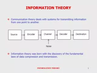
Change to an efficient representation,i.e., data compression. Change to an efficient representation for,transmission, i.e., error control coding. Channel Any source of information Source Channel Channel coder Source coder Source decoder Sink, receiver Channel decoder Recover from channel distortion. Uncompress The channel is anything transmitting or storing information –a radio link, a cable, a disk, a CD, a piece of paper, …
Channel Source Channel Channel coder Source coder Source decoder Sink, receiver Channel decoder Fundamental Entities H R C C H: The information content of the source. R: Rate from the source coder. C: Channel capacity.
Channel Source Channel Channel decoder Channel coder Source coder Source decoder Sink, receiver Source coding theorem (simplified) Channel coding theorem (simplified) Fundamental Theorems H R C C Shannon 1: Error-free transmission possible if R¸H and C¸R. Shannon 2: Source coding and channel coding can be optimized independently, and binary symbols can be used as intermediate format. Assumption: Arbitrarily long delays.
Source X1, X2, … Part 2: Stochastic sources • A source outputs symbolsX1, X2, ... • Each symbol take its value from an alphabetA= (a1, a2, …). • Model:P(X1,…,XN) assumed to be known for all combinations. Example 1: A text is a sequence of symbols each taking its value from the alphabetA= (a, …, z, A, …, Z, 1, 2, …9, !, ?, …). Example 2: A (digitized) grayscale image is a sequence of symbols each taking its value from the alphabet A= (0,1) or A= (0, …, 255).
Two Special Cases • The Memoryless Source • Each symbol independent of the previous ones. • P(X1, X2, …, Xn) = P(X1) ¢P(X2) ¢ … ¢P(Xn) • The Markov Source • Each symbol depends on the previous one. • P(X1, X2, …, Xn)= P(X1) ¢P(X2|X1) ¢P(X3|X2) ¢ … ¢P(Xn|Xn-1)
b 0.7 a 0.5 1.0 0.3 c 0.2 0.3 The Markov Source • A symbol depends only on the previous symbol, so the source can be modelled by a state diagram. A ternary source withalphabet A= (a, b, c).
The Markov Source • Assume we are in state a, i.e., Xk = a. • The probabilities for the next symbol are: b 0.7 P(Xk+1 = a | Xk = a) = 0.3P(Xk+1 =b | Xk = a) = 0.7P(Xk+1 = c | Xk = a) = 0 a 0.5 1.0 0.3 c 0.2 0.3
b 0.7 P(Xk+2 = a | Xk+1 = b) = 0P(Xk+2 =b | Xk+1 = b) = 0P(Xk+2 = c | Xk+1 = b) = 1 a 0.5 1.0 0.3 c 0.2 0.3 The Markov Source • So, if Xk+1 = b, we know that Xk+2 willequal c.
The Markov Source • If all the states can be reached, the stationary probabilities for the states can be calculated from the given transition probabilities. • Markov models can be used to represent sources with dependencies more than one step back. • Use a state diagram with several symbols in each state. Stationary probabilities? That’s theprobabilities i= P(Xk = ai) for anyk when Xk-1, Xk-2, … are not given.
Analysis and Synthesis • Stochastic models can be used for analysing a source. • Find a model that well represents the real-world source, and then analyse the model instead of the real world. • Stochastic models can be used for synthesizing a source. • Use a random number generator in each step of a Markov model to generate a sequence simulating the source.
Part 3: Information and Entropy • Assume a binary memoryless source, e.g., a flip of a coin. How much information do we receive when we are told that the outcome is heads? • If it’s a fair coin, i.e., P(heads) = P (tails) = 0.5, we say that the amount of information is 1 bit. • If we already know that it will be (or was) heads, i.e., P(heads) = 1, the amount of information is zero! • If the coin is not fair, e.g., P(heads) = 0.9, the amount of information is more than zero but less than one bit! • Intuitively, the amount of information received is the same if P(heads) = 0.9 or P (heads) = 0.1.
Self Information • So, let’s look at it the way Shannon did. • Assume a memoryless source with • alphabet A= (a1, …, an) • symbol probabilities (p1, …, pn). • How much information do we get when finding out that the next symbol is ai? • According to Shannon the self information of ai is
Why? Assume two independent eventsA and B, withprobabilities P(A) = pA and P(B) = pB. For both the events to happen, the probability ispA¢ pB. However, the amount of informationshould be added, not multiplied. Logarithms satisfy this! No, we want the information to increase withdecreasing probabilities, so let’s use the negativelogarithm.
Example 2: Self Information Example 1: Which logarithm? Pick the one you like! If you pick the natural log,you’ll measure in nats, if you pick the 10-log, you’ll get Hartleys,if you pick the 2-log (like everyone else), you’ll get bits.
On average over all the symbols, we get: Self Information H(X) is called the first order entropy of the source. This can be regarded as the degree of uncertaintyabout the following symbol.
Often denoted Let BMS 0 1 1 0 1 0 0 0 … Then 1 The uncertainty (information) is greatest when 0 0.5 1 Entropy Example:Binary Memoryless Source
Entropy: Three properties • It can be shown that 0 ·H·log N. • Maximum entropy (H = log N) is reached when all symbols are equiprobable, i.e.,pi = 1/N. • The difference log N – H is called the redundancy of the source.
Part 4: Entropy for Memory Sources • Assume a block of source symbols (X1, …, Xn) and define the block entropy: • The entropy for a memory source is defined as: That is, the summation is done over all possible combinations of n symbols. That is, let the block length go towards infintity.Divide by n to get the number of bits / symbol.
Pkl is the transition probability from state k to state l. Entropy for a Markov Source The entropy for a state Sk can be expressed as Averaging over all states, we get theentropy for the Markov source as
A B 1- 1- The Run-length Source • Certain sources generate long runs or bursts of equal symbols. • Example: • Probability for a burst of length r: P(r) = (1-)r-1¢ • Entropy: HR = - r=11P(r) logP(r) • If the average run length is , then HR/ = HM.
Part 5: The Source Coding Theorem The entropy is the smallest number of bitsallowing error-free representation of the source. Why is this? Let’s take a look on typical sequences!
Typical Sequences • Assume a long sequence from a binary memoryless source with P(1) = p. • Among n bits, there will be approximatelyw = n ¢ pones. • Thus, there is M = (n over w) such typical sequences! • Only these sequences are interesting. All other sequences will appear with smaller probability the larger is n.
bits/symbol Enumeration needs log Mbits, i.e, bits per symbol! How many are the typical sequences?
How many bits do we need? Thus, we need H(X) bits per symbolto code any typical sequence!
The Source Coding Theorem • Does tell us • that we can represent the output from a source X using H(X) bits/symbol. • that we cannot do better. • Does not tell us • how to do it.
Summary • The mathematical model of communication. • Source, source coder, channel coder, channel,… • Rate, entropy, channel capacity. • Information theoretical entities • Information, self-information, uncertainty, entropy. • Sources • BMS, Markov, RL • The Source Coding Theorem