3. Work Hardening Models

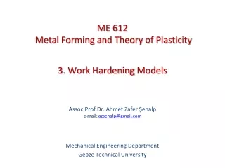
1. ME 612 Metal Forming and Theory of Plasticity 3. WorkHardeningModels Assoc.Prof.Dr. Ahmet Zafer Şenalpe-mail: azsenalp@gmail.com Mechanical Engineering Department Gebze Technical University

2. 3. WorkHardeningModels In this section work hardening models that are applicable to different materials and metal forming operations are covered. For correct model selection material experiment results and specifications of metal forming operation should be considered. Mechanical Engineering Department, GTU

3. 3.1. PerfectlyElastic Model 3. WorkHardeningModels In the below figure stress-strain curve of a perfectly elastic material is shown. For this model Hook’s law; İs valid. Brittle materials like glass, ceramic and some of the cast irons can be modeled with this model. For materials that have short rupture elongation (% 1...2) and goes to rupture immediately after yield point perfectly elastic model is used. (3.1) Figure 3.1. Perfectly elastic model Mechanical Engineering Department, GTU

4. 3.2. RigidPerfectlyPlastic Model 3. WorkHardeningModels No hardening, plastic material model. In the below figure rigid perfectly plastic model of an ideal material is shown. A tensile specimen of this model is rigid until tensile stress reaches to yield point (elastic deformation is zero). When tensile stress reaches to yield point plastic deformation starts and deformation continues under constant stress (without work hardening). Figure 3.2. Rigid perfectly plastic model Mechanical Engineering Department, GTU

5. 3.3. RigidLinearWorkHardening Model 3. WorkHardeningModels In the below figure true stress-true strain diagram of a rigid linear work hardening material is given. In such a material deformation is not observed until tensile stress reaches to yield point. When tensile stress reaches to yield point plastic deformation starts and in order to increase deformation stress should be increased also. In this model stress varies linearly with plastic strain (linear work hardening). As in rigid perfectly plastic model elastic deformation is neglected in this model. This model is applied to plastic bending analysis of beams. Figure 3.3. Rigid linear work hardening model Mechanical Engineering Department, GTU

6. 3.4. ElasticPerfectlyPlastic Model 3. WorkHardeningModels In the below figure true stress-true strain diagram of a elastic perfectly plastic material is shown. Figure 3.4. Elastic perfectly plastic model Mechanical Engineering Department, GTU

7. 3.5. ElasticLinearWorkHardening Model 3. WorkHardeningModels This model shows elastic linear hardening behaviour. Figure 3.5. Elastic linear work hardening model Mechanical Engineering Department, GTU

8. 3.6. LudwigPowerLaw 3. WorkHardeningModels Some empirical equations that fit to the experimentally obtained true stress-true strain curves have been developed. One of them is developed by Ludwig and valid in constant temperature and strain rate situations; Here ; Y: Yield strength H: Material dependent strength coefficient n: Work hardening power. (3.2) Figure 3.6. Ludwig power law Mechanical Engineering Department, GTU

9. 3.6. LudwigPowerLaw 3. WorkHardeningModels For different work hardening power values different stress-strain curve generates. These can be summarized as: • n = 1 case: the equation represents a material which is rigid up to the yield stress Y, followed by deformation at a constant strain­hardening rate H. It may be applied to cold-worked materials and gives an especially good fit for 'half-hard' aluminium. Figure 3.7. Ludwig power law and n = 1 case Mechanical Engineering Department, GTU

10. 3.6. LudwigPowerLaw 3. WorkHardeningModels • n < 1 case: In this caseelastic component of the strain is neglected. After yield point material work hardens however due to plastic deformation there is no linear relation between stress and strain (work hardening is not linear). Mechanical Engineering Department, GTU

11. 3.6. LudwigPowerLaw 3. WorkHardeningModels • n < 1 andY = O case (Figure 3.8): If Y=0 is placed in Ludwig equation different form of Ludwig equation is obtained; Such a material does not show an elastic behavior from the beginning of loading and yield point is not evident. (3.3) Figure 3.8. Different form of Ludwig law; (Y=0) Mechanical Engineering Department, GTU

12. 3.6. LudwigPowerLaw 3. WorkHardeningModels In the below table H and n values for various materials are given. Table 3.1. H and n values for various materials at room temperature Mechanical Engineering Department, GTU

13. 3.7. Swift PowerLaw 3. WorkHardeningModels The work hardening law recommended by Swift is; B: Prestrain coefficient n: Work hardening power. n is a measure of work hardening. If n is high work hardenening is high, if n is low work hardenening is less. C: is a function of direction of stress. Especially for operations that have large deformation Swift law yields results closer to the reality. But it is more complex than other models. (3.4) Figure 3.9. Swift curve Mechanical Engineering Department, GTU

14. 3.7. Swift PowerLaw 3. WorkHardeningModels Figure 3.10 Swift curve for B=0 Mechanical Engineering Department, GTU

15. 3.8. TemperatureEffect 3. WorkHardeningModels The above Swift equation can be rearranged to include temperature effects. : related with cold forming. : related with hot forming, : work hardening coefficient, : work softening coefficient, n : work hardening power m : work softening power (3.5) Mechanical Engineering Department, GTU

16. 3.9. DeterminingtheParameters in WorkHardeningLaw 3. WorkHardeningModels To determine which work hardening model to use it is necessary to make experiments. To determine the type of the experiment the operation should be investigated. This subject will be covered in the advancing chapters. After the experiment true stress-true strain graph should be plotted. The next step is to choose appropriate work hardening law that fits to the plot in hand. Here let’s assume that the below work hardening law is selected. Here it is explained how to compute K and n parameters. To determine these parameters it is necessary to plot work hardening power law in logarithmic scale. (3.6) Mechanical Engineering Department, GTU

17. 3.9. DeterminingtheParameters in WorkHardeningLaw 3. WorkHardeningModels Or in mathematical form; Linear equation is obtained. If work hardening law İs choosen linear equation is obtained. Experimental points are placed in this equation and diagram inFigure 3.11. is obtained . Here the slope of the line gives “n” value and log σ valuecorresponding to log=0value yieldslogK value. (3.7) (3.8) (3.9) (3.10) Figure 3.11. log versus log σ diagram Mechanical Engineering Department, GTU

18. 3.9. DeterminingtheParameters in WorkHardeningLaw 3. WorkHardeningModels Similar solutions can be applied toor to other work hardening laws. In Figure 3.12 true tress-true strain graphs of some materials and in Figure 3.13’ logarithmic plots are shown. Figure 3.13. True tress-true strain graphs of some materials in logarithmic scale. Figure 3.12. True tress-true strain graphs of some materials (Trans. ASM,46,998, 1954). Mechanical Engineering Department, GTU