Particle Physics
This course covers the practicalities of particle physics, including textbooks, course outline, natural units, 4-vector notation, study of decays and reactions, and Feynman diagrams. Contact details and office hours provided.

Particle Physics
E N D
Presentation Transcript
Particle Physics Nikos Konstantinidis
Practicalities (I) • Contact details • My office: D16, 1st floor Physics, UCL • My e-mail: n.konstantinidis@ucl.ac.uk • Web page: www.hep.ucl.ac.uk/~nk/teaching/PH4442 • Office hours for the course (this term) • Tuesday 13h00 – 14h00 • Friday 12h30 – 13h30 • Problem sheets • To you at week 1, 3, 5, 7, 9 • Back to me one week later • Back to you (marked) one week later
Practicalities (II) • Textbooks • I recommend (available for £23 – ask me or Dr. Moores) • Griffiths “Introduction to Elementary Particles” • Alternatives • Halzen & Martin “Quarks & Leptons” • Martin & Shaw “Particle Physics” • Perkins “Introduction to High Energy Physics” • General reading • Greene “The Elegant Universe”
Course Outline • Introduction (w1) • Symmetries and conservation laws (w2) • The Dirac equation (w3) • Electromagnetic interactions (w4,5) • Strong interactions (w6,7) • Weak interactions (w8,9) • The electroweak theory and beyond (w10,11)
Week 1 – Outline • Introduction: elementary particles and forces • Natural units, four-vector notation • Study of decays and reactions • Feynman diagrams/rules & first calculations
The matter particles • All matter particles (a) have spin ½; (b) are described by the same equation (Dirac’s); (c) have antiparticles • Particles of same type but different families are identical, except for their mass: me = 0.511MeV mm=105.7MeV mt=1777MeV • Why three families? Why they differ in mass? Origin of mass? • Elementary a point-like (…but have mass/charge/spin!!!)
The force particles • All force particles have spin 1 (except for the graviton, still undiscovered, expected with spin 2) • Many similarities but also major differences: • mg = 0 vs. mW,Z~100GeV • Unlike photon, strong/weak “mediators” carry their “own charge” • The SM provides a unified treatment of EM and Weak forces (and implies the unification of Strong/EM/Weak forces); but requires the Higgs mechanism (→ the Higgs particle, still undiscovered!).
Natural Units • SI units not “intuitive” in Particle Physics; e.g. • Mass of the proton ~1.7×10⁻²⁷kg • Max. momentum of electrons @ LEP ~5.5×10⁻¹⁷kg∙m∕sec • Speed of muon in pion decay (at rest) ~8.1×10⁷m∕sec • More practical/intuitive: ħ = c =1; this means energy, momentum, mass have same units • E2 = p2 c2 + m2 c4 E2 = p2 + m2 • E.g. mp=0.938GeV, max. pLEP=104.5GeV, vm=0.27 • Also: • Time and length have units of inverse energy! • 1GeV-1 =1.973×10⁻¹⁶m 1GeV-1 =6.582×10⁻²⁵sec
4-vector notation (I) Lorentz Transformations 4-vector: “An object that transforms like xm between inertial frames” E.g. Invariant: “A quantity that stays unchanged in all inertial frames” E.g. 4-vector scalar product: 4-vector length: Length can be: >0 timelike <0 spacelike =0 lightlike 4-vector
4-vector notation (II) • Define matrix g: g00=1, g11=g22=g33=-1 (all others 0) • Also, in addition to the standard 4-v notation (contravariant form: indices up), define covariant form of 4-v (indices down): • Then the 4-v scalar product takes the tidy form: • An unusual 4-v is the four-derivative: • So, ∂mam is invariant; e.g. the EM continuity equation becomes:
What do we study? • Particle Decays (AB+C+…) • Lifetimes, branching ratios etc… • Reactions (A+BC+D+…) • Cross sections, scattering angles etc… • Bound States • Mass spectra etc…
Study of Decays (AB+C+…) • Decay rate G: “The probability per unit time that a particle decays” • Lifetime t: “The average time it takes to decay” (at particle’s rest frame!) • Usually several decay modes • Branching ratio BR • We measure Gtot (or t) and BRs; we calculate Gi
Nmax G 0.5Nmax M0 G as decay width • Unstable particles have no fixed mass due to the uncertainty principle: • The Breit-Wigner shape: • We are able to measure only one of G, t of a particle ( 1GeV-1 =6.582×10⁻²⁵ sec )
Study of reactions (A+BC+D+…) • Cross section s • The “effective” cross-sectional area that A sees of B (or B of A) • Has dimensions L2 and is measured in (subdivisions of) barns 1b = 10-28 m2 1mb = 10-34 m2 1pb = 10-40 m2 • Often measure “differential” cross sections • ds/dW or ds/d(cosq) • Luminosity L • Number of particles crossing per unit area and per unit time • Has dimensions L-2T-1; measured in cm-2s-1 (1031 – 1034)
Study of reactions (cont’d) • Event rate (reactions per unit time) • Ordinarily use “integrated” Luminosity (in pb-1) to get the total number of reactions over a running period • In practice, L measured by the event rate of a reaction whose s is well known (e.g. Bhabha scattering at LEP: e+e– e+e–). Then cross sections of new reactions are extracted by measuring their event rates
Feynman diagrams • Feynman diagrams: schematic representations of particle interactions • They are purely symbolic! Horizontal dimension is (…can be) time (except in Griffiths!) but the other dimension DOES NOT represent particle trajectories! • Particle going backwards in time => antiparticle forward in time • A process A+BC+D is described by all the diagrams that have A,B as input and C,D as output. The overall cross section is the sum of all the individual contributions • Energy/momentum/charge etc are conserved in each vertex • Intermediate particles are “virtual” and are called propagators; The more virtual the propagator, the less likely a reaction to occur • Virtual:
Fermi’s “Golden Rule” • Calculation of G or s has two components: • Dynamical info: (Lorentz Invariant) Amplitude (or Matrix Element) M • Kinematical info: (L.I.) Phase Space (or Density of Final States) • FGR for decay rates (12+3+…+n) • FGR for cross sections (1+23+4+…+n)
Feynman rules to extract M Toy theory: A, B, C spin-less and only ABC vertex • Label all incoming/outgoing 4-momenta p1, p2,…, pn; Label internal 4-momenta q1, q2…,qn. • Coupling constant: for each vertex, write a factor –ig • Propagator: for each internal line write a factor i/(q2–m2) • E/p conservation: for each vertex write (2p)4d4(k1+k2+k3); k’s are the 4-momenta at the vertex (+/– if incoming/outgoing) • Integration over internal momenta: add 1/(2p)4d4q for each internal line and integrate over all internal momenta • Cancel the overall Delta function that is left: (2p)4d4(p1+p2–p3…–pn) What remains is:
Summary • The SM particles & forces [1.1->1.11, 2.1->2.3] • Natural Units • Four-vector notation [3.2] • Width, lifetime, cross section, luminosity [6.1] • Fermi’s G.R. and phase space for 1+2–>3+4 [6.2] • Mandelstam variables [Exercises 3.22, 3.23] • d-functions [Appendix A] • Feynman Diagrams [2.2] • Feynman rules for the ABC theory [6.3] • ds/dW for A+B–>A+B [6.5] • Renormalisation, running coupling consts [6.6, 2.3]