Time Averaging
Time Averaging. Steven A. Jones BIEN 501 Monday, April 14, 2008. Time Averaging. Major Learning Objectives: Apply time averaging to the momentum and energy transport equations. Time Averaging. Minor Learning Objectives: Define a time average. State reasons for time averaging.

Time Averaging
E N D
Presentation Transcript
Time Averaging Steven A. Jones BIEN 501 Monday, April 14, 2008 Louisiana Tech University Ruston, LA 71272
Time Averaging Major Learning Objectives: • Apply time averaging to the momentum and energy transport equations. Louisiana Tech University Ruston, LA 71272
Time Averaging Minor Learning Objectives: • Define a time average. • State reasons for time averaging. • Demonstrate how linearity and nonlinearity affect time averaging. • Demonstrate the main rules for time averaging. • Compare time averaging to linear filtering. • Time average the momentum equation. • Describe Reynolds stresses. • Time average the energy equation. • Describe turbulent energy flux. Louisiana Tech University Ruston, LA 71272
Definition of a Time Average If we have a variable, such as velocity, we can define the time average of that variable as: What is t? What is Dt? How can u(t) be a function of time if it is time-averaged? Louisiana Tech University Ruston, LA 71272
Definition of a Time Average Time averaging is a special case of a linear (low pass) filter (moving average). Where W(t) is a weighting window. You should recognize this form as a convolution (or cross-correlation) between the weighting function and the variable of interest. Louisiana Tech University Ruston, LA 71272
What are t andDt? The definition is a moving average, and t is the time at which the window is applied. Dt In this example, Dt is 10 msec. Louisiana Tech University Ruston, LA 71272
Long Time/Short Time When we talk about u(t), t is referred to as short time. When we talk about , t is referred to as long time. Louisiana Tech University Ruston, LA 71272
Why Time Average? • We may be interested in changes that occur over longer periods of time. • We may want to filter out noise in a signal. • Measurements are often filtered. All instruments have some kind of time constant. • Examples: • Do weather patterns suggest global warming? • What is the overall flow rate from a piping system? • What is the average shear stress to which an endothelial cell is subjected? Louisiana Tech University Ruston, LA 71272
Continuity and Linearity The equation of continuity is: The time average is: If density is constant: When an equation is linear, the time average for the equation can be found simply by substituting the time averaged variable for the time dependent variable. E.g. incompressible continuity is and time-averaged incompressible continuity is . Louisiana Tech University Ruston, LA 71272
Consequences of Linearity The time average of a derivative is the derivative of a time average. The same result holds for time derivatives: Louisiana Tech University Ruston, LA 71272
Time Averaged Time Average From linear systems, a signal filtered twice is different from a signal filtered once, as can readily be seen from the frequency domain. But if the slow fluctuations are sufficiently separated in frequency from the fast fluctuations, the average of the average is approximately the same as the average. In particular, for fluctuations in steady flow, the two averages are the same. Louisiana Tech University Ruston, LA 71272
Sample “Steady Flow” Data Disturbed Turbulent In each case, what is the “time average?” Louisiana Tech University Ruston, LA 71272
Is This Flow Disturbed? What is the correct averaging time? Louisiana Tech University Ruston, LA 71272
Choices • We need to determine what time frame we are interested. The time frame is determined by the value of Dt. • How does the earth’s rotation affect temperature? (Dt ~ hours) • How does the earth’s tilt affect weather? (Dt ~ days) • How does the earth’s magnetic field affect weather? (Dt ~ years) Louisiana Tech University Ruston, LA 71272
Consequences of Nonlinearity The time average of a product is not the product of time averages. We will often divide a variable into two components, one of which is constant and one of which is time variant. The time average becomes simply . Louisiana Tech University Ruston, LA 71272
Consequences of Nonlinearity With , since it follows that . The time average of the product becomes: Louisiana Tech University Ruston, LA 71272
Additional Relationships Louisiana Tech University Ruston, LA 71272
Additional Relationships Louisiana Tech University Ruston, LA 71272
Additional Relationships Louisiana Tech University Ruston, LA 71272
Additional Relationships Louisiana Tech University Ruston, LA 71272
Time Averaged Momentum Consider the z1 Momentum Equation in the form. Let r be constant and let: Then: Louisiana Tech University Ruston, LA 71272
Time Averaged Momentum The equation Looks like the non time-averaged version, except for the extra terms: Louisiana Tech University Ruston, LA 71272
Time Averaged Momentum Consider these terms, and apply the product rule for differentiation (in reverse): Then: Louisiana Tech University Ruston, LA 71272
Time Averaged Momentum Rearrange: Then the term in parentheses is: Which is zero by continuity. Louisiana Tech University Ruston, LA 71272
Time Averaged Momentum Now take the time average: To get: Louisiana Tech University Ruston, LA 71272
Time Averaged Momentum The terms: Look like the divergence of a second order tensor defined by: Consequently, it is customary to write the time averaged momentum equations in the form: Louisiana Tech University Ruston, LA 71272
Reynolds Stresses • Have the form of a stress tensor. • Act as true stresses on the mean flow. • Are referred to in the biomedical engineering literature relating cell damage and platelet activation to turbulence. • But are not the stresses directly imposed on the cells. (Viscous shearing). Louisiana Tech University Ruston, LA 71272
Reynolds Stresses • If an eddy of fluid suddenly move through the velocity field: The fluid would tend to change the local momentum. • Thus, the Reynolds Stress is not a shear upon the fluid itself, only upon the velocity field. • THIS IS A VERY IMPORTANT DISTINCTION Louisiana Tech University Ruston, LA 71272
Reynolds Stresses • Cell Damage • Since cells such as Red Blood Cells (RBC), monocytes, and platelets can be affected by shearing, it is important to determine the degree of shearing to which a cell is subjected in a given flow geometry. • This is particularly important in regions of turbulence such as downstream of a stenosed valve or downstream of tight vascular constrictions. Louisiana Tech University Ruston, LA 71272
Reynolds Stresses – 2D Flow • If the rate of strain is given as follows: • Then we can write the energy extracted from the mean flow and converted to turbulent fluctuations due to strain rate as: Louisiana Tech University Ruston, LA 71272
Reynolds Stresses – 2D Flow • The energy which is extracted from the turbulent kinetic energy and converted to heat through viscous shearing is called viscous dissipation and is designated by ε Louisiana Tech University Ruston, LA 71272
Reynolds Stresses – 2D Flow • Then in homogeneous steady flow such that • It follows that over the entire turbulent region, Louisiana Tech University Ruston, LA 71272
Reynolds Stresses – 2D Flow • There are several mechanisms that can damage blood cells. Two of these are pressure fluctuations and shear stress. • Pressure fluctuations are generally more important for larger particles since a net shear on the particle requires a difference in pressure along its length. • Shearing is a more likely mechanism for damage in cells the size of RBC. Louisiana Tech University Ruston, LA 71272
Reynolds Stresses – 2D Flow • The Reynolds Stresses, , are often used as a measure of the stresses on the individual cells. • Even though are called Reynolds Shearing Stresses, they do not represent the shearing stresses on individual cells. • Rather, they are the stresses on the mean flow field, as stated before. Louisiana Tech University Ruston, LA 71272
Reynolds Stresses – 2D Flow • It is, however, much easier to measure the Reynolds Stresses than it is to measure the viscous dissipation • Because the Reynolds Stresses occur over a much larger scale than the viscous stresses. • Thus, we use this identity to estimate the viscous dissipation, and thus total stresses on the flow from the Reynolds Stresses. How would you measure the Reynolds Stresses? Louisiana Tech University Ruston, LA 71272
Time Averaged Energy Equation Louisiana Tech University Ruston, LA 71272
Time Averaged Energy Equation From: The cross terms between time averaged and fluctuating values again become zero. So: Louisiana Tech University Ruston, LA 71272
Time Averaged Energy Equation From: Apply the product rule: (Incompressible) Same as in book because: So Louisiana Tech University Ruston, LA 71272
Use of Turbulent Energy Flux • Solutions to the energy equation depend on finding empirical and semi-theoretical relations for the turbulent energy flux. • Turbulent energy flux will depend on temperature gradient and the stress tensor. • Turbulence tends to transport energy, momentum and mass through mixing. I.e. turbulence carries things across “mean streamlines” and distributes them more evenly. Louisiana Tech University Ruston, LA 71272