Download
1 / 13
130 likes | 240 Vues
This document summarizes the preliminary results from the first phase of the PILPS-C1 experiment, conducted at the Loobos EUFLUX site, which features a mature coniferous forest. The project analyzed biophysical and biogeochemical fluxes, including NEE, LE, H, and Rn, comparing model outputs with observed data from 1997-1998. Future work will include additional simulations, parameter calibrations, and deeper insights into carbon dynamics. Key participants from various institutes collaborated in the project, marking significant advancements in understanding forest carbon fluxes.

E N D
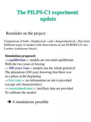
The PILPS-C1 experiment • Results of the first phase of the project • Complementary simulation to be done • Proposition for the future
Summary of the first phase of the project Comparison of both « biophysical » and « biogeochemical » flux from Different types of models with observations at one EUROFLUX site: Loobos • The site: • Temperate « mature(100 years) » coniferous forest • Climate: 700 mm precipitation , 9.8 °C mean temperature • Planted on a sand no soil carbon at the beginning of the plantation • Measured fluxes: NEE, LE,H, Rn • Meteorological parameters: incoming SW rad., precipitation, • temperature, wind speed, relative humidity, pressure • -Period covered: 1997-1998 Models: Including SVAT with and without carbon cycle • Proposed simulations: • Free equilibrium simulations: • Models are run until equilibrium of state variables using years 1997-1998 • « in loop » • Free 100 years run: • simulation of « realistic scenario »: Beginning with a soil with no • Carbon, the models are run for 1906 (plantation of the forest) to 1998 • Using observed climate. • Constrained equilibrium simulations: • Same as free equilibrium but with calibrations of parameters • (simulation delayed…)
PILPSC1 workshop The workshop was held from May 6-7 2003 at CNRS center in Gif-sur-Yvette, France. Support for the workshop was provided by CNRS/INSU. The participants of the workshop where: Jean Christophe Calvet (CNRM, France), Yeugeniy Gusev (Institute of Water Problems, Russia), Mustapha El Mayaar (Univ. Wisconsin,USA) Eddy Moors (Alterra, Netherlands), Olga Nasanova (Institute of Water Problems, Russia), Jan Polcher (LMD, France), Vincent Rivalland (CNRM, France), Andrey Shmakin (Institute of Geography, Russia), Diana Verseghy (CCS, Canada), Nicolas Viovy (LSCE,France)
Main results « free equilibrium simulation » Analysis on diurnal cycle, daily and monthly average • For each models: • Plots of mean diurnal cycles over 10 days • Plots of mean seasonal diurnal cycles • Plots of daily and monthly means • Plots of monthly model v.s data • Global statistics: • intercept v.s. Slope • RMSE sys v.s. non systematic: • The RMSE systematic indicate « bias » in the model • The RMSE non-systematic is the residue of the RMSE • Index of agreement: Global measurement of agreement between • model an observation.
Slope/intercept and RMSE unsys/sys For the different models (3 hourly fluxes)
« 100 years simulation » • Same as for F-E run plus: • Comparison of sinks simulated and observed for 1997 and 1998 • Trajectories of several parameters for the 93 years of the run: • NEE • GPP • NPP • Total soil carbon • Total living biomass • biomass increment
Modeled and simulated carbon net sink In 1997 and 1998
Annual NEE (Kg C m-2 y-1) Annual GPP (Kg C m-2 y-1) CLASS-MCM CLASS-UA CLASS-MCM CLASS-UA ORCHIDEE-1 ORCHIDEE-1 ORCHIDEE-2 ORCHIDEE-2 IBIS SWAP IBIS AVIM MC 2 kind of behaviors: IBIS of ORCHIDEE-1 that reach rapidly the NPP (beginning with High sink) CLASS or SWAP with progressive increase of NPP (with increasing sink) MC or ORCHIDEE-2 is between the two.
Total Soil carbon (Kg C/m-2) Total living biomass (Kg C/m-2) CLASS-MCM CLASS-UA CLASS-MCM CLASS-UA ORCHIDEE-1 ORCHIDEE-1 ORCHIDEE-2 ORCHIDEE-2 SWAP SWAP VISA VISA MC IBIS IBIS MC AVIM AVIM
Completion of the first phase (end of 2003...) New model outputs will be added e.g: LAI, separation between below and above Biomass, height of trees..... • Calibrated simulations with: • LAI (trees, understorey(seasonal cycle) • Maximun unstressed assimilation • Root zone depth • Water table depth • Height of trees (height of « first branches ») • Litter layer • Soil carbon (to check if we can informations about partition between pools) • Soil water content • Soil temperature Some new analysis Separation between night/day cloudy/clear warm/cold Estimation of WUE Ratio NEE/total respiration.
Main preliminary conclusion Taking into account that models was not calibrated The models reproduce relatively well the observations Sensible heat flux is overestimated at night High net CO2 and latent heat fluxes are underestimated The 100 years simulation was very interesting Since if all models give relatively similar NEE And are all able to reproduce the difference of Sink between 1997 and 1998, trajectories of Models carbon fluxes and pools are very different ! For more details on results go to: http://www.pilpsc1.cnrs-gif.fr