Lecture 1 Introduction to Electronics

1. Lecture 1Introduction to Electronics This material is adapted from Chapter 1 “Microelectronic Circuit Design” by Richard C. Jaeger, Travis N. Blalock McGraw Hill

2. Goals • Explore the history of electronics. • Impact of integrated circuit technologies. • Describe classification of electronic signals. • Review circuit notation and theory.

3. The Start of the Modern Electronics Era Bardeen, Shockley, and Brattain at Bell Labs - Brattain and Bardeen invented the bipolar transistor in 1947. The first germanium bipolar transistor. Roughly 50 years later, electronics account for 10% (4 trillion dollars) of the world GDP.

4. Braun invents the solid-state rectifier. DeForest invents triode vacuum tube. 1907-1927 First radio circuits de-veloped from diodes and triodes. 1925 Lilienfeld field-effect device patent filed. Bardeen and Brattain at Bell Laboratories invent bipolar transistors. Commercial bipolar transistor production at Texas Instruments. Bardeen, Brattain, and Shockley receive Nobel prize. Integrated circuit developed by Kilby and Noyce First commercial IC from Fairchild Semiconductor IEEE formed from merger or IRE and AIEE First commercial IC opamp One transistor DRAM cell invented by Dennard at IBM. 4004 Intel microprocessor introduced. First commercial 1-kilobit memory. 1974 8080 microprocessor introduced. Megabit memory chip introduced. 2000 Alferov, Kilby, and Kromer share Nobel prize Electronics Milestones

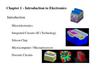
5. Evolution of Electronic Devices Vacuum Tubes Discrete Transistors SSI and MSI Integrated Circuits VLSI Surface-Mount Circuits

6. Microelectronics Proliferation • The integrated circuit was invented in 1958. • World transistor production has more than doubled every year for the past twenty years. • Every year, more transistors are produced than in all previous years combined. • Approximately 109 transistors were produced in a recent year. • Roughly 50 transistors for every ant in the world . *Source: Gordon Moore’s Plenary address at the 2003 International Solid State Circuits Conference.

7. Device Feature Size • Feature size reductions enabled by process innovations. • Smaller features lead to more transistors per unit area and therefore higher density.

8. Rapid Increase in Density of Microelectronics Memory chip density versus time. Microprocessor complexity versus time.

9. Signal Types • Analog signals take on continuous values - typically current or voltage. • Digital signals appear at discrete levels. Usually we use binary signals which utilize only two levels. • One level is referred to as logical 1 and logical 0 is assigned to the other level.

10. Analog signals are continuous in time and voltage or current. (Charge can also be used as a signal conveyor.) After digitization, the continuous analog signal becomes a set of discrete values, typically separated by fixed time intervals. Analog and Digital Signals

11. For an n-bit D/A converter, the output voltage is expressed as: The smallest possible voltage change is known as the least significant bit or LSB. Digital-to-Analog (D/A) Conversion

12. Analog input voltage vx is converted to the nearest n-bit number. For a four bit converter, 0 -> vx input yields a 0000 -> 1111 digital output. Output is approximation of input due to the limited resolution of the n-bit output. Error is expressed as: Analog-to-Digital (A/D) Conversion

13. Notational Conventions • Total signal = DC bias + time varying signal • Resistance and conductance - R and G with same subscripts will denote reciprocal quantities. Most convenient form will be used within expressions.

14. What are Reasonable Numbers? • If the power suppy is +/-10 V, a calculated DC bias value of 15 V (not within the range of the power supply voltages) is unreasonable. • Generally, our bias current levels will be between 1 uA and a few hundred milliamps. • A calculated bias current of 3.2 amps is probably unreasonable and should be reexamined (except in power devices). • Peak-to-peak ac voltages should be within the power supply voltage range. • A calculated component value that is unrealistic should be rechecked. For example, a resistance equal to 0.013 ohms. • Given the inherent variations in most electronic components, three significant digits are adequate for representation of results.

15. and Combining these yields the basic voltage division formula: Circuit Theory Review: Voltage Division Applying KVL to the loop, and

16. Circuit Theory Review: Voltage Division (cont.) Using the derived equations with the indicated values, Design Note: Voltage division only applies when both resistors are carrying the same current.

17. where and Combining and solving for vs, Combining these yields the basic current division formula: Circuit Theory Review: Current Division and

18. Circuit Theory Review: Current Division (cont.) Using the derived equations with the indicated values, Design Note: Current division only applies when the same voltage appears across both resistors.

19. Circuit Theory Review: Thevenin and Norton Equivalent Circuits

20. Problem: Find the Thevenin equivalent voltage at the output. Solution: Known Information and Given Data: Circuit topology and values in figure. Unknowns: Thevenin equivalent voltage vTH. Approach: Voltage source vTH is defined as the output voltage with no load. Assumptions: None. Analysis: Next slide… Circuit Theory Review: Find the Thevenin Equivalent Voltage

21. Circuit Theory Review: Find the Thevenin Equivalent Voltage Applying KCL at the output node, Current i1 can be written as: Combining the previous equations

22. Circuit Theory Review: Find the Thevenin Equivalent Voltage (cont.) Using the given component values: and

23. Problem: Find the Thevenin equivalent resistance. Solution: Known Information and Given Data: Circuit topology and values in figure. Unknowns: Thevenin equivalent voltage vTH. Approach: Voltage source vTH is defined as the output voltage with no load. Assumptions: None. Analysis: Next slide… Circuit Theory Review: Find the Thevenin Equivalent Resistance Test voltage vx has been added to the previous circuit. Applying vx and solving for ix allows us to find the Thevenin resistance as vx/ix.

24. Circuit Theory Review: Find the Thevenin Equivalent Resistance (cont.) Applying KCL,

25. Frequency Spectrum of Electronic Signals • Nonrepetitive signals have continuous spectra often occupying a broad range of frequencies • Fourier theory tells us that repetitive signals are composed of a set of sinusoidal signals with distinct amplitude, frequency, and phase. • The set of sinusoidal signals is known as a Fourier series. • The frequency spectrum of a signal is the amplitude and phase components of the signal versus frequency.

26. Frequencies of Some Common Signals • Audible sounds 20 Hz - 20 KHz • Baseband TV 0 - 4.5 MHz • FM Radio 88 - 108 MHz • Television (Channels 2-6) 54 - 88 MHz • Television (Channels 7-13) 174 - 216 MHz • Maritime and Govt. Comm. 216 - 450 MHz • Cell phones 1710 - 2690 MHz • Satellite TV 3.7 - 4.2 GHz

27. Fourier Series • Any periodic signal contains spectral components only at discrete frequencies related to the period of the original signal. • A square wave is represented by the following Fourier series: 0=2/T (rad/s) is the fundamental radian frequency and f0=1/T (Hz) is the fundamental frequency of the signal. 2f0, 3f0, 4f0 and called the second, third, and fourth harmonic frequencies.

28. Amplifier Basics • Analog signals are typically manipulated with linear amplifiers. • Although signals may be comprised of several different components, linearity permits us to use the superposition principle. • Superposition allows us to calculate the effect of each of the different components of a signal individually and then add the individual contributions to the output.

29. Amplifier Input/Output Response vs = sin2000t V Av = -5 Note: negative gain is equivalent to 180 degress of phase shift.

30. Introduction to ElectronicsFall 2010 Electric Circuits Analysis of linear circuits • Thevenin ‘s Theorem • Norton ‘s Theorem • Superposition • Equivalent circuits • Controlled sources • Introduction to Electronics • Operational amplifier non-idealities • Diodes, BJT & MOS transistors as nonlinear elements • The CMOS and BJT as Amplifiers and as Digital Inverters • Generating device linear model for using in analysis and simulations • Bandwidth estimation, frequency response • Multi-stage amplifier circuits • Digital circuits basics • Analog to digital conversion basics