Introduction to Thermodynamic Diagrams
390 likes | 995 Vues
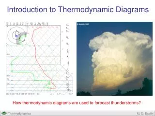
Introduction to Thermodynamic Diagrams. How thermodynamic diagrams are used to forecast thunderstorms?. Introduction to Thermodynamic Diagrams. Outline: Basic Idea of Thermodynamic Diagrams Possible Diagrams Skew-T Log-P Diagram Rawinsondes Dropsondes Skew-T Applications.

Introduction to Thermodynamic Diagrams
E N D
Presentation Transcript
Introduction to Thermodynamic Diagrams How thermodynamic diagrams are used to forecast thunderstorms? M. D. Eastin
Introduction to Thermodynamic Diagrams • Outline: • Basic Idea of Thermodynamic Diagrams • Possible Diagrams • Skew-T Log-P Diagram • Rawinsondes • Dropsondes • Skew-T Applications M. D. Eastin
Basic Idea of Thermodynamic Diagrams • Advantages: • A visualization tool • We can always use the mathematical formulas… • Many of us learn better through visualization… • Eliminates or simplifies the equations • Can determine many quantities in a graphical format • Desired Qualities in a Thermodynamic Diagram: • 1. For cyclic processes, the area should be proportional to the work done • or the heat exchanged • 2. The lines should be straight (easy to use) • 3. The angle between adiabats and isotherms should be as large as possible • (easy to distinguish variations in atmospheric stability→ will air rise or sink) • (more on stability later…) M. D. Eastin
Possible Thermodynamic Diagrams • P-V Diagrams? • Pros: • Satisfies Requirement #1 • Good for illustrating basic concepts • Cons: • Angle between isotherms and • adiabats is very small • Isotherms and adiabats are not • straight lines • We don’t observe volume • We need to use a different diagram • that satisfies all three requirements • and uses a coordinate system for • observable variables p Isobar i Isochor Adiabat f Isotherm V M. D. Eastin
W P A V B Basic Idea of Thermodynamic Diagrams • Area-Equivalent Transformations: • P-V diagrams only satisfy Requirement #1: Enclosed area proportional to energy • Thus, we need to consider other variables for the coordinate systems • Create a generic transformation from P, V → A, B M. D. Eastin
WpV WAB P A V B Basic Idea of Thermodynamic Diagrams Area-Equivalent Transformations: M. D. Eastin
Temperature -20oC -40oC 400 mb 60oC qe 0oC 40oC 600 mb Pressure 20oC 800 mb w q = 0oC 1000 mb Possible Thermodynamic Diagrams • Tephigram: • Area proportional to energy • 3 sets of nearly straight lines • Isotherms (T) • Adiabats (θ) • Saturation Mixing Ratio (w) • Isobars (p) are curved • Pseudo-adiabats (θe) are curved • 90º angle between adiabats • and isotherms Note: We will talk about the pseudo-adiabats (θe) and saturation mixing ratio (w) lines later in the course M. D. Eastin
400 mb 100oC 80oC qe 60oC 600 mb 40oC Pressure 20oC w 800 mb q = 0oC -20oC 1000 mb 40oC -40oC -20oC 0oC 20oC Temperature Possible Thermodynamic Diagrams • Emagram: • Area proportional to energy • 4 sets of nearly straight lines • Isobars (p) • Isotherms (T) • Adiabats (θ) • Saturation Mixing Ratio (w) • Pseudo-adiabats (θe) are curved • 45º angle between adiabats • and isotherms Note: We will talk about the pseudo-adiabats (θe) and saturation mixing ratio (w) lines later in the course M. D. Eastin
Possible Thermodynamic Diagrams • Skew-T Log-P Diagram: • Area proportional to energy • 3 sets of nearly straight lines • Isobars (p) • Isotherms (T) • Saturation Mixing Ratio (w) • Adiabats (θ) are slightly curved • Pseudo-adiabats (θe) are curved • ~90º angle between adiabats • and isotherms See Example on Next Slide Note: We will talk about the pseudo-adiabats (θe) and saturation mixing ratio (w) lines later in the course M. D. Eastin
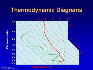
200 -10 300 0 Pressure (mb) 400 10 20 500 30 600 40 700 800 900 1000 Temperature (oC) Possible Thermodynamic Diagrams Skew-T Log-P Diagram: Isobars (p) Isotherms (T) Saturation Mixing Ratio (w) Adiabats (θ) Pseudo-adiabats (θe) M. D. Eastin
The Skew-T Log-P Diagram • Skew-T Log-P Diagram: • Most commonly used diagram (we will use it too…) • Come in a variety of shapes, sizes, and colors. • All Skew-T Log-P diagrams provide the exact same information! M. D. Eastin
The Skew-T Log-P Diagram Note how the lines of constant temperature slope (or are skewed) toward the upper left Hence, “Skew-T” These lines are always solid and straight but vary in color Our Version: Red solid lines M. D. Eastin
The Skew-T Log-P Diagram Note how the change in pressure along the Y-axis in non-uniform Rather, it changes logarithmically Hence, “Log-P” These lines are always solid and straight but may vary in color Our Version: Blue solid lines M. D. Eastin
The Skew-T Log-P Diagram The dry adiabats, or lines of constant potential temperature slope at almost right angles to the isotherms These lines are always solid and slightly curved, but may vary in color Our Version: Light Blue Solid Lines M. D. Eastin
The Skew-T Log-P Diagram The lines of constant saturation mixing ratio are also skewed toward the upper left More on these in a future lecture… These lines are always dashed and straight, but may vary in color Our Version: Pink dashed Lines M. D. Eastin
Skew-T Applications The saturation adiabats are lines of constant equivalent potential temperature and they represent pseudo- adiabatic processes More on these in a future lecture… These lines are always dashed and curved, but may vary in color Our Version: Dashed bluish-green M. D. Eastin
Skew-T Log-P Diagram Pressure (200 mb) Pseudo-Adiabat (283K) Dry Adiabat (283K) Isotherm (T=-10ºC) Saturation Mixing Ratio (10 g/kg) 10ºC = 283K M. D. Eastin
Skew-T Log-P Diagram Plot Rawinsonde or Dropsonde Observations: Temperature Dewpoint Temperature M. D. Eastin
The Rawinsonde • Instrument Package attached to a Balloon: • Launched twice daily (00 and 12 UTC) • Regular launch locations • Rise from the surface into the stratosphere before the balloon bursts • Observe pressure (p), temperature (T), dewpoint temperature (Td), • altitude (z), and horizontal winds (speed, direction) at numerous • regular levels through the atmosphere. Temperature and Humidity Sensor M. D. Eastin
The Global Rawinsonde Network Standard 1200 UTC Rawinsonde Sites M. D. Eastin
The Dropsonde • Instrument Package attached to a Parachute: • Launched from aircraft or hot air balloons • over data sparse regions (e.g. the oceans) • Used to improve “high-impact” forecasts • Hurricane forecasts • Winter storm forecasts • Irregular launch times and locations • Fall the from launching platform down to • the surface using a parachute that • controls the rate of descent • Observe pressure (p), temperature (T), • dewpoint (Td), altitude (z), and horizontal • winds (speed, direction) at numerous • regular levels through the atmosphere. M. D. Eastin
Skew-T Applications Identify Temperature Inversions Inversions are layers where temperature increases with height M. D. Eastin
Skew-T Applications Identify Dry Adiabatic Layers Dry-adiabatic layers have the temperature profile parallel to a dry adiabat M. D. Eastin
Skew-T Applications Determine the Potential Temperature (θ) of any Air Parcel Bring air parcel down a dry-adiabat to 1000 mb Add 273 K to the T-value Begin with parcel at 400 mb T = 40ºC θ = 313 K M. D. Eastin
Introduction to Thermodynamic Diagrams • Summary: • Basic Idea of Thermodynamic Diagrams • Possible Diagrams • Skew-T Log-P Diagram • Rawinsondes • Dropsondes • Skew-T Applications M. D. Eastin
References Petty, G. W., 2008: A First Course in Atmospheric Thermodynamics, Sundog Publishing, 336 pp. Tsonis, A. A., 2007: An Introduction to Atmospheric Thermodynamics, Cambridge Press, 197 pp. Wallace, J. M., and P. V. Hobbs, 1977: Atmospheric Science: An Introductory Survey, Academic Press, New York, 467 pp. Also (from course website): NWSTC Skew-T Log-P Diagram and Sounding Analysis, National Weather Service, 2000 The Use of the Skew-T Log-P Diagram in Analysis and Forecasting, Air Weather Service, 1990 M. D. Eastin