Survey Networks Project Planning: Geodetic Data Corrections & Standards

1. Class 25: Even More Corrections and Survey Networks Project Planning 21 April 2008

2. Deadlines • Reading assignments (2) due 30 April 2008 • Sample of what I expect is posted to class wiki page • Extra credit due 23 April 2008 • No lab assignments/homework will be accepted after today.

3. Textbook • EM 1110-1-1003, Chapters 4-10 • Geodesy text, Chapter 11

4. Does distance matter in GPS? Article available on NGS web site http://www.ngs.noaa.gov/CORS/Articles/

6. Plumb line • Indicates the average direction of gravity between the point of suspension and the plumb bob. • It is perpendicular to every each level surface it intersects. • Equipotential surfaces are NOT parallel • Effected by mass of the earth • Oceans are a mass deficiency • Mountains a mass concentration

7. Astro-Geodetic

9. Deflection of the Vertical Angle between the plumb line and a normal to the ellipsoid is the deflection of the vertical. City of Corpus Christi, TX Ft. Davis, TX Denali, AK

10. Computation of Deflection • Has a North South component ξ (xi) and East West component η(eta) • Computed with respect to astronomical azimuth (A) • ξ = θ cos A and η = θ sin A • Positive ξ indicates astronomic latitude will fall north of the geodetic latitude • Positiveη indicates astronomic longitude will fall east of geodetic longitude

11. http://www.exploretheline.com/

13. Mason-Dixon Line  = Φ - ξ

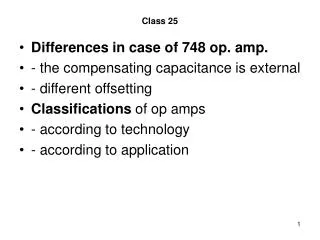
14. Distance Corrections • Refraction – may be overcome by reciprocal vertical/zenith angles • Otherwise: k is coefficient of atmospheric refraction R is mean earth radius hA is ellipsoid height of instrument station

15. Curvature Correction • Accounts for the fact that plumb lines are not parallel at different locations on earth’s surface.

16. Geodetic Distance • Computed from level distance (LD) • LD * [ R / (R + h) ] • LD * [ R / (R + H + N) ] • Use R = 6,371,000 m • H = Orthometric Height • h = ellipsoid height • N = geoid height

17. Planning GPS Control Surveys • Your plan will be developed in accordance with your client’s goals and the relevant standards. • EM 1110-1-1003 describes work for the USACE. • These differ from FGCS standards and specifications.

18. Issues in Any Plan • Project Datum • Mostly will be NAD 83 (but which version?) • Intended accuracy • Horizontal, Vertical or both • Which height system (ellipsoidal or NAVD 88) • More accuracy = More $$$$ • Monumentation • Equipment needed (and available)

19. Project Planning/Standards and Specifications • See class page for links to relevant documents.

28. Meeting standards • We must have redundant observations in order to evaluate their precision. • We must have ties to fixed control (more than one) in order to attach our observations to this framework as well as to verify the relationship of the fixed points. • When our observations are more accurate than the fixed network, we degrade them to fit the network.

29. Level Data Reduction and Adjustment 5

30. Leveling summary

31. Populating the design matrix • Height difference (i to j) is equal to the observed difference and its residual/variance. • Line 1. D – A = 1.978 + variance • Line 2. E – A = 0.732 + v • Line 3. D – C = 0.988 + v • Line 4. E – B = 0.420 + v • Line 5. D – E = 1.258 + v

32. Design Matrix (Free) “From” station gets a “-1” “To” station gets a “1”

33. Note diagonal elements!

34. Observations/Distances

35. Account for Known BMs • Review diagram • Solve for heights where direct connection to unknown 5

36. Updated Matrices

37. Rearrange to put BMs on right side • D = 11.999 + v • E = 10.753 + v • D = 11.990 + v • E = 10.741 + v • D – E = 1.258 + v

38. Why not just mean heights? How do we account for the difference in elevation from E to D? How accurate is our result?

39. Matlab Un-weighted Result Calculate residuals Calculate heights

40. Weight Matrix • We assume that error will accumulate as a function of distance. • Weights assigned as 1/distKM.

41. Weight Matrix • P used for weight matrix (also W) • Diagonal Matrix assumes no correlations • Applied to both design matrix and observation matrix • X = ATPA-1*ATPL

42. D = 11.9976 E = 10.7445

43. Differences in Results