Download
1 / 59
600 likes | 929 Vues
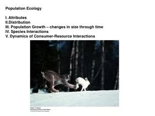
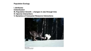
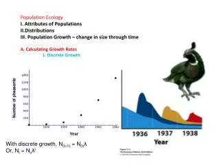
Population Ecology Attributes of Populations Distributions III. Population Growth – change in size through time Calculating Growth Rates 1. Discrete Growth. With discrete growth, N (t+1) = N (t) λ Or, N t = N o λ t. Population Ecology Attributes of Populations Distributions

E N D
Population Ecology • Attributes of Populations • Distributions • III. Population Growth – change in size through time • Calculating Growth Rates • 1. Discrete Growth With discrete growth, N(t+1) = N(t)λ Or, Nt = Noλt
Population Ecology • Attributes of Populations • Distributions • III. Population Growth – change in size through time • Calculating Growth Rates • 2. Exponential Growth – continuous reproduction With discrete growth: N(t+1) = N(t)λ or Nt = Noλt Continuous growth: Nt = Noert Where r = intrinsic rate of growth (per capita and instantaneous) and e = base of natural logs (2.72) So, λ = er
If λ is between zero and 1, the r < 0 and the population will decline. • If λ = 1, then r = 0 and the population size will not change. • If λ >1, then r > 0 and the population will increase. • Population Ecology • Attributes of Populations • Distributions • III. Population Growth – change in size through time • Calculating Growth Rates • 3. Equivalency
The rate of population growth is measured as: The derivative of the growth equation: Nt = Noert dN/dt = rNo • Population Ecology • Attributes of Populations • Distributions • III. Population Growth – change in size through time • Calculating Growth Rates • 3. Equivalency
III. Population Growth – change in size through time • Calculating Growth Rates B. The Effects of Age Structure 1. Life Table - static: look at one point in time and survival for one time period
III. Population Growth – change in size through time • Calculating Growth Rates B. The Effects of Age Structure 1. Life Table
III. Population Growth – change in size through time • Calculating Growth Rates B. The Effects of Age Structure 1. Life Table Why λ ? (discrete breeding season and discrete time intervals)
III. Population Growth – change in size through time • Calculating Growth Rates B. The Effects of Age Structure 1. Life Table - dynamic (or “cohort”) – follow a group of individuals through their life Song Sparrows Mandarte Isl., B.C. (1988)
Age classes (x): x = 0, x = 1, etc. Initial size of the population: nx, at x = 0.
Age classes (x): x = 0, x = 1, etc. Initial size of the population: nx, at x = 0. Number reaching each birthday are subsequent values of nx
Age classes (x): x = 0, x = 1, etc. Initial size of the population: nx, at x = 0. Survivorship (lx): proportion of population surviving to age x.
Age classes (x): x = 0, x = 1, etc. Initial size of the population: nx, at x = 0. Survivorship (lx): proportion of population surviving to age x. Mortality: dx = # dying during interval x to x+1. Mortality rate: mx = proportion of individuals age x that die during interval x to x+1.
Survivorship Curves: Describe age-specific probabilities of survival, as a consequence of age-specific mortality risks.
Age classes (x): x = 0, x = 1, etc. Initial size of the population: nx, at x = 0. Survivorship (lx): proportion of population surviving to age x. Number alive DURING age class x: Lm = (nx + (nx+1))/2
Age classes (x): x = 0, x = 1, etc. Initial size of the population: nx, at x = 0. Survivorship (lx): proportion of population surviving to age x. Number alive DURING age class x: Lm = (nx + (nx+1))/2 Expected lifespan at age x = ex - T = Sum of Lm's for age classes = , > than age (for 3, T = 9) - ex = T/nx (number of individuals in the age class) ( = 9/12 = 0.75) - ex = the number of additional age classes an individual can expect to live.
III. Population Growth – change in size through time • Calculating Growth Rates B. The Effects of Age Structure 1. Life Tables 2. Age Class Distributions
III. Population Growth – change in size through time • Calculating Growth Rates B. The Effects of Age Structure 1. Life Tables 2. Age Class Distributions When these rates equilibrate, all age classes are growing at the same single rate – the intrinsic rate of increase of the population (rm)
III. Population Growth – change in size through time • Calculating Growth Rates • B. The Effects of Age Structure • C. Growth Potential Net Reproductive Rate = Σ(lxbx) = 2.1 Number of daughters/female during lifetime. If it is >1 (“replacement”), then the population has the potential to increase multiplicatively (exponentially).
III. Population Growth – change in size through time • Calculating Growth Rates • B. The Effects of Age Structure • C. Growth Potential Generation Time – T = Σ(xlxbx)/ Σ(lxbx) = 1.95
III. Population Growth – change in size through time • Calculating Growth Rates • B. The Effects of Age Structure • C. Growth Potential Intrinsic rate of increase: rm (estimated) = ln(Ro)/T = 0.38 Pop growth dependent on reproductive rate (Ro) and age of reproduction (T).
III. Population Growth – change in size through time • Calculating Growth Rates • B. The Effects of Age Structure • C. Growth Potential Intrinsic rate of increase: rm (estimated) = ln(Ro)/T = 0.38 Pop growth dependent on: reproductive rate (Ro) and age of reproduction (T). Doubling time = t2 = ln(2)/r = 0.69/0.38 = 1.82 yrs
III. Population Growth – change in size through time • Calculating Growth Rates • B. The Effects of Age Structure • C. Growth Potential Northern Elephant Seals: <100 in 1900 150,000 in 2000. r = 0.073, λ = 1.067 Malthus: All populations have the capacity to expand exponentially
III. Population Growth – change in size through time • Calculating Growth Rates • B. The Effects of Age Structure • C. Growth Potential • D. Life History Redux R = 10 T = 1 r = 2.303 Net Reproductive Rate = Σ(lxbx) = 10 Generation Time – T = Σ(xlxbx)/ Σ(lxbx) = 1.0 rm (estimated) = ln(Ro)/T = 2.303
III. Population Growth – change in size through time • Calculating Growth Rates • B. The Effects of Age Structure • C. Growth Potential • D. Life History Redux • - increase fecundity, increase growth rate (obvious) R = 10 T = 1 r = 2.303 R = 11 T = 1 r = 2.398
III. Population Growth – change in size through time • Calculating Growth Rates • B. The Effects of Age Structure • C. Growth Potential • D. Life History Redux • - increase fecundity, increase growth rate (obvious) • - decrease generation time (reproduce earlier) – increase growth rate R =11 T = 1 r = 2.398 R = 12 T = 0.833 r = 2.983
III. Population Growth – change in size through time • Calculating Growth Rates • B. The Effects of Age Structure • C. Growth Potential • D. Life History Redux • - increase fecundity, increase growth rate (obvious) • - decrease generation time (reproduce earlier) – increase growth rate • - increasing survivorship – DECREASE GROWTH RATE (lengthen T) R = 11 T = 1 r = 2.398 R = 20 T = 1.5 r = 2.00
III. Population Growth – change in size through time • Calculating Growth Rates • B. The Effects of Age Structure • C. Growth Potential • D. Life History Redux • - increase fecundity, increase growth rate (obvious) • - decrease generation time (reproduce earlier) – increase growth rate • - increasing survivorship – DECREASE GROWTH RATE (lengthen T) • - survivorship adaptive IF: • - necessary to reproduce at all • - by storing E, reproduce disproportionately in the future R = 230 T = 2.30 r = 2.36 Original r = 2.303
III. Population Growth – change in size through time • Calculating Growth Rates • B. The Effects of Age Structure • C. Growth Potential • D. Life History Redux • E. Limits on Growth: Density Dependence Robert Malthus 1766-1834
Premise: - as population density increases, resources become limiting and cause an increase in mortality rate, a decrease in birth rate, or both... r > 0 DEATH BIRTH RATE r < 0 DENSITY
Premise: - as population density increases, resources become limiting and cause an increase in mortality rate, a decrease in birth rate, or both... r > 0 RATE r < 0 DEATH BIRTH DENSITY
Premise: - as population density increases, resources become limiting and cause an increase in mortality rate, a decrease in birth rate, or both... r > 0 r < 0 DEATH RATE BIRTH DENSITY
As density increases, successful reproduction declines And juvenile suvivorship declines (mortality increases)
Lots of little plants begin to grow and compete. This kills off most of the plants, and only a few large plants survive.
Premise: Result: There is a density at which r = 0 and DN/dt = 0. THIS IS AN EQUILIBRIUM.... r = 0 DEATH RATE BIRTH DENSITY K
Premise • 2. Result • 3. The Logistic Growth Equation: • Exponential: • dN/dt = rN N t
Premise • 2. Result • 3. The Logistic Growth Equation: • Exponential: Logistic: • dN/dt = rNdN/dt = rN [(K-N)/K] K N N t t
Premise • 2. Result • 3. The Logistic Growth Equation (Pearl-Verhulst Equation, 1844-45): • Logistic: • dN/dt = rN [(K-N)/K] When a population is very small (N~0), the logistic term ((K-N)/K) approaches K/K (=1) and growth rate approaches the exponential maximum (dN/dt = rN). K N t
Premise • 2. Result • 3. The Logistic Growth Equation: • Logistic: • dN/dt = rN [(K-N)/K] As N approaches K, K-N approaches 0; so that the term ((K-N)/K) approaches 0 and dN/dt approaches 0 (no growth). K N t
Premise • 2. Result • 3. The Logistic Growth Equation: • Logistic: • dN/dt = rN [(K-N)/K] Should N increase beyond K, K-N becomes negative, as does dN/dt (the population will decline in size). K N t
Premise • 2. Result • 3. The Logistic Growth Equation: • Logistic: • dN/dt = rN [(K-N)/K] [(N-m)/K] Minimum viable population size add (N-m)/N K N m t
III. Population Growth – change in size through time • Calculating Growth Rates • B. The Effects of Age Structure • C. Growth Potential • D. Life History Redux • E. Limits on Growth: Density Dependence • F. Temporal Dynamics
F. Temporal Dynamics - DISCRETE GROWTH ROUGHLY, growth per generation is: log(Nt+1) - log(Nt) = R[log(K) - log(Nt)] SO: when R < 1, the population will grow only a fraction of the difference between K and Nt. Asymptotic approach to K. K N Nt t
F. Temporal Dynamics - DISCRETE GROWTH ROUGHLY, growth per generation is: log(Nt+1) - log(Nt) = R[log(K) - log(Nt)] SO: If R = 1, then the population reaches K exactly. K N Nt t
F. Temporal Dynamics - DISCRETE GROWTH ROUGHLY, growth per generation is: log(Nt+1) - log(Nt) = R[log(K) - log(Nt)] SO: If 1.0 < R < 2.0, then the population overshoots by progressively smaller amounts... convergent oscillation. K N Nt t
SO: If 1.0 < R < 2.0, then the population overshoots by progressively smaller amounts... convergent oscillation. K N Nt t
SO: If 1.0 < R < 2.0, then the population overshoots by progressively smaller amounts... convergent oscillation. K N Nt t
F. Temporal Dynamics - DISCRETE GROWTH ROUGHLY, growth per generation is: log(Nt+1) - log(Nt) = R[log(K) - log(Nt)] SO: when 2 < R < 2.5, oscillations increase each time interval; divergent oscillation initially. But at low N, the linearity breaks down and this equation is not descriptive. End up with a stable limit cycle.Over 2.5? Chaotic. K N Nt t
F. Temporal Dynamics - DISCRETE GROWTH
F. Temporal Dynamics - CONTINUOUS GROWTH Breed here, and may be out of balance with resources Lags occur because of developmental time between acquisition of resources FOR breeding and the event of breeding itself. K N Nt t