Optimality Proof of A* Search Heuristics
Learn about the admissibility of A*, cycle checking, and constructing heuristics for optimal path finding in search algorithms. Understand the optimal efficiency and effect of search heuristics in A* algorithms.

Optimality Proof of A* Search Heuristics
E N D
Presentation Transcript
A* optimality proof, cycle checking CPSC 322 – Search 5 Textbook § 3.6 and 3.7.1 January 21, 2011 Taught by Mike Chiang
Lecture Overview • Recap • Admissibility of A* • Cycle checking and multiple path pruning
Searchheuristics Def.: A search heuristic h(n) is an estimate of the cost of the optimal (cheapest) path from node n to a goal node. • Think of h(n) as only using readily obtainable (easy to compute) information about a node. • h can be extended to paths: • h(n0,…,nk)=h(nk) Def.: A search heuristic h(n) is admissible if it never overestimates the actual cost of the cheapest path from a node to the goal
How to Construct a Heuristic • Identify relaxed version of the problem: • where one or more constraints have been dropped • problem with fewer restrictions on the actions Result: The cost of an optimal solution to the relaxed problem is an admissible heuristic for the original problem(because it is always weakly less costly to solve a less constrained problem!)
Example 2 Search problem: robot has to find a route from start to goal location on a grid with obstacles Actions: move up, down, left, right from tile to tile Cost : number of moves Possible h(n)? Manhattan distance (L1 distance) between two points sum of the (absolute) difference of their coordinates 4 3 2 1 G 1 2 3 4 5 6
Example 2 Search problem: robot has to find a route from start to goal location on a grid with obstacles Actions: move up, down, left, right from tile to tile Cost : number of moves Possible h(n)? Would the Euclidian distance (straight line distance be an admissible heuristic? 4 3 2 1 G 1 2 3 4 5 6
Would the Euclidean distance (straight line distance) be an admissible heuristic for the robot grid problem? It is an admissible search heuristic It is a search heuristic, but it is not admissible It is not a suitable search heuristic for this problem
A* Search • A* search takes into account both • the cost of the path to a node c(p) • the heuristic value of that path h(p). • Let f(p) = c(p) + h(p). • estimate of the cost of a path from the start to a goal via p. • A* always chooses the path on the frontier with the lowest estimated distance from the start to a goal node constrained to go via that path. c(p) h(p) f(p)
Lecture Overview • Recap of Lecture 8 • Admissibility of A* • Cycle checking and multiple path pruning
Admissibility of A* • A* is complete (finds a solution, if one exists) and optimal (finds the optimal path to a goal) if: • the branching factor is finite • arc costs are > 0 • h(n) is admissible -> an underestimate of the length of the shortest path from n to a goal node. • This property of A* is called admissibility of A*
Why is A* admissible: complete • It halts (does not get caught in cycles) because: • Let fmin be the cost of the optimal solution path s(unknown but finite if there exists a solution) • Each sub-path p of s has cost f(p) ≤ fmin • Due to admissibility (exercise: prove this at home) • Let fmin > 0 be the minimal cost of any arc • All paths with length > fmin / cmin have cost > fmin • A* expands path on the frontier with minimal f(n) • Always a prefix of s on the frontier • Only expands paths p with f(p) ≤ fmin • Terminates when expanding s • See how it works on the “misleading heuristic” problem in AI space:
Why is A* admissible: optimal • Let p* be the optimal solution path, with cost c*. • Let p’ be a suboptimal solution path. That is c(p’) > c*. • We are going to show that any sub-path p’’ of p* on the frontier will be expanded before p’ => A* won’t be caught by p’ p” p’ p*
Analysis of A* • If fact, we can prove something even stronger about A* (when it is admissible) • A* is optimally efficient among the algorithms that extend the search path from the initial state. • It finds the goal with the minimum # of expansions
Why A* is Optimally Efficient • No other optimal algorithm is guaranteed to expand fewer nodes than A* • This is because any algorithm that does not expand every node with f(n) < f* risks to miss the optimal solution
Effect of Search Heuristic • A search heuristic that is a better approximation on the actual cost reduces the number of nodes expanded by A* • Example: 8puzzle • tiles can move anywhere • (h1 : number of tiles that are out of place) • tiles can move to any adjacent square • (h2 : sum of number of squares that separate each tile from its correct position) • average number of paths expanded: (d = depth of the solution) • d=12 BFS = 3,644,035 paths A*(h1) = 227 paths A*(h2) = 73 paths • d=24 BFS = too many paths A*(h1) = 39,135 paths A*(h2) = 1,641 paths
Time Space Complexity of A* • Time complexity is O(bm) • the heuristic could be completely uninformative and the edge costs could all be the same, meaning that A* does the same thing as BFS • Space complexity is O(bm) like BFS, A* maintains a frontier which grows with the size of the tree
Learning Goals for today’s class • Formally prove A* optimality • Define optimally efficient • Construct admissible heuristics for specific problems.
Lecture Overview • Recap of Lecture 8 • Admissibility of A* • Cycle checking and multiple path pruning
Cycle Checking • You can prunea node nthat is on the path from the start node to n. • This pruning cannot remove an optimal solution => cycle check • What is the computational cost of cycle checking?
Computational Cost of Cycle Checking? Constant time: set a bit to 1 when a node is selected for expansion, and never expand a node with a bit set to 1 Linear time in the path length: before adding a new node to the currently selected path, check that the node is not already part of the path It depends on the algorithm None of the above