Interpolation - Introduction
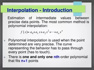
Interpolation - Introduction. Estimation of intermediate values between precise data points. The most common method is polynomial interpolation:

Interpolation - Introduction
E N D
Presentation Transcript
Interpolation - Introduction Estimation of intermediate values between precise data points. The most common method is polynomial interpolation: • Polynomial interpolation is used when the point determined are very precise. The curve representing the behavior has to pass through every point (has to touch). • There is one and only onenth-order polynomial that fits n+1 points
Introduction n = 3 n = 4 n = 2 First order (linear) 2nd order (quadratic) 3rd order (cubic)
Interpolation Polynomials are the most common choice of interpolation because they are easy to: • Evaluate • Differentiate, and • Integrate. 3
Introduction There are a variety of mathematical formats in which this polynomial can be expressed: • The Newton polynomial (sec. 18.1) • The Lagrange polynomial (sec. 18.2)
Newton’s Divided-Difference Interpolating Polynomials Linear Interpolation/ • Is the simplest form of interpolation, connecting two data points with a straight line. • f1(x) designates that this is a first-order interpolating polynomial. Slope and a finite divided difference approximation to 1st derivative Linear-interpolation formula
Figure 18.2
Quadratic Interpolation/ • If three data points are available, the estimate is improved by introducing some curvature into the line connecting the points. • A simple procedure can be used to determine the values of the coefficients.
General Form of Newton’s Interpolating Polynomials/ Bracketed function evaluations are finite divided differences
Lagrange Interpolating Polynomials • The general form for n+1 data points is: designates the “product of”
Lagrange Interpolating Polynomials • Linear version (n = 1): Used for 2 points of data: (xo,f(xo)) and (x1,f(x1)),
Lagrange Interpolating Polynomials • Second order version (n = 2):
Lagrange Interpolating Polynomials - Example Use a Lagrange interpolating polynomial of the first and second order to evaluate ln(2) on the basis of the data:
Lagrange Interpolating Polynomials – Example (cont’d) • First order polynomial:
Lagrange Interpolating Polynomials – Example (cont’d) • Second order polynomial:
Coefficients of an Interpolating Polynomial • Although “Lagrange” polynomials are well suited for determining intermediate values between points, they do not provide a polynomial in conventional form: • Since n+1data points are required to determine n+1 coefficients, simultaneous linear systems of equations can be used to calculate “a”s.
Coefficients of an Interpolating Polynomial (cont’d) Where “x”s are the knowns and “a”s are the unknowns.
Why Spline Interpolation? Apply lower-order polynomials to subsets of data points. Spline provides a superior approximation of the behavior of functions that have local, abrupt changes. 20
Spline Interpolation • Polynomials are the most common choice of interpolants. • There are cases where polynomials can lead to erroneous results because of round off error and overshoot. • Alternative approach is to apply lower-order polynomials to subsets of data points. Such connecting polynomials are called spline functions.
Why Splines ? Figure : Higher order polynomial interpolation is a bad idea 23
Spline Interpolation The concept of spline is using a thin , flexible strip (called a spline) to draw smooth curves through a set of points….natural spline (cubic)
Linear Spline The first order splines for a group of ordered data points can be defined as a set of linear functions:
x f(x) 3.0 2.5 4.5 1.0 7.0 2.5 9.0 0.5 Linear spline - Example Fit the following data with first order splines. Evaluate the function at x = 5.
Linear Spline • The main disadvantage of linear spline is that they are not smooth. The data points where 2 splines meets called (a knot), the changes abruptly. • The first derivative of the function is discontinuous at these points. • Using higher order polynomial splines ensure smoothness at the knots by equating derivatives at these points.
Quadric Splines • Objective: to derive a second order polynomial for each interval between data points. • Terms:Interior knots and end points For n+1 data points: • i = (0, 1, 2, …n), • n intervals, • 3n unknown constants (a’s, b’s and c’s)
Quadric Splines (3n conditions) • The function values of adjacent polynomial must be equal at the interior knots 2(n-1). • The first and last functions must pass through the end points (2).
Quadric Splines (3n conditions) • The first derivatives at the interior knots must be equal (n-1). • Assume that the second derivate is zero at the first point (1) (The first two points will be connected by a straight line)
Quadric Splines - Example Fit the following data with quadratic splines. Estimate the value at x = 5. Solutions: There are 3 intervals (n=3), 9 unknowns.
Quadric Splines - Example • Equal interior points: • For first interior point (4.5, 1.0) The 1st equation: The 2nd equation:
Quadric Splines - Example • For second interior point (7.0, 2.5) The 3rd equation: The 4th equation:
Quadric Splines - Example • First and last functions pass the end points For the start point (3.0, 2.5) For the end point (9, 0.5)
Quadric Splines - Example • Equal derivatives at the interior knots. For first interior point(4.5, 1.0) For second interior point(7.0, 2.5) • Second derivative at the first point is 0
Quadric Splines - Example Solving these 8 equations with 8 unknowns
Cubic Splines Objective: to derive a third order polynomial for each interval between data points. Terms:Interior knots and end points For n+1 data points: • i = (0, 1, 2, …n), • n intervals, • 4n unknown constants (a’s, b’s ,c’s and d’s)
Cubic Splines (4n conditions) • The function values must be equal at the interior knots (2n-2). • The first and last functions must pass through the end points (2). • The first derivatives at the interior knots must be equal (n-1). • The second derivatives at the interior knots must be equal (n-1). • The second derivatives at the end knots are zero (2), (the 2nd derivative function becomes a straight line at the end points)
Alternative technique to get Cubic Splines • The second derivative within each interval [xi-1, xi] is a straight line. (the 2nd derivatives can be represented by first order Lagrange interpolating polynomials. A straight line connecting the first knot f’’(xi-1) and the second knot f’’(xi) The second derivative at any point x within the interval
Cubic Splines • The last equation can be integrated twice 2 unknown constants of integration can be evaluated by applying the boundary conditions: 1. f(x) = f (xi-1)atxi-1 2. f(x) = f (xi)atxi Unknowns: i = 0, 1,…, n
Cubic Splines • For each interior point xi(n-1): This equation result with n-1 unknown second derivatives where, for boundary points: f˝(xo) = f˝(xn) = 0
Cubic Splines - Example Fit the following data with cubic splines Use the results to estimate the value at x=5. Solution: • Natural Spline:
Cubic Splines - Example • For 1st interior point (x1 = 4.5) - - - Apply the following equation:
Cubic Splines - Example Since • For 2nd interior point (x2 = 7 )
Cubic Splines - Example Apply the following equation: Since
Cubic Splines - Example Solve the two equations: The first interval (i=1), apply for the equation:
Cubic Splines - Example The 2nd interval (i =2), apply for the equation: The 3rd interval (i =3), For x= 5:
Credits: • Chapra, Canale • The Islamic University of Gaza, Civil Engineering Department