Prevalence of Color Blindness among Drivers in a State: Results of a Z-Test
100 likes | 124 Vues
This text summarizes the results of a z-test conducted to determine if the proportion of color blind drivers in a random sample of 1000 licensed drivers is significantly different from 20% at a significance level of 0.05.

Prevalence of Color Blindness among Drivers in a State: Results of a Z-Test
E N D
Presentation Transcript
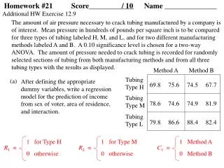
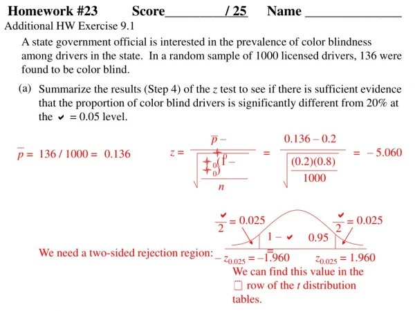
Homework #23 Score____________ / 25 Name ______________ Additional HW Exercise 9.1 (a) A state government official is interested in the prevalence of color blindness among drivers in the state. In a random sample of 1000 licensed drivers, 136 were found to be color blind. Summarize the results (Step 4) of the z test to see if there is sufficient evidence that the proportion of color blind drivers is significantly different from 20% at the = 0.05 level. p – 0 0.136 – 0.2 z = = = – 5.060 p = 136 / 1000 = 0.136 0(1 – 0) ———— n (0.2)(0.8) ———— 1000 — = 2 0.025 — = 2 0.025 1 – = 0.95 We need a two-sided rejection region: – z0.025 = –1.960 z0.025 = 1.960 We can find this value in the row of the t distribution tables.
Since z = have sufficient evidence to reject H0 . We conclude that – 5.060and z0.025 = 1.960, we the proportion of color blind drivers is different from 20%. (P < 0.001). The data suggest that this proportion is less than 20%. The two-sided P-value can be found from the t distribution tables.
Additional HW Exercise 9.1.-continued (b) Considering the results of the hypothesis test in part (a), explain why it would be of interest to find a confidence interval for the proportion of color blind drivers; then find a 95% confidence interval for this proportion. Since rejecting H0 leads us to conclude that the proportion is different from 20%, a confidence interval provides some information about the size of the difference. p (1 –p) ———— n p (1 –p) ———— n p– z/2 and p+ z/2 — = 2 0.025 — = 2 0.025 1 – = 0.95 – z0.025 = 1.960 z0.025 = 1.960 0.136(1 –0.136) ——————— 1000 0.136(1 –0.136) ——————— 1000 0.136– 1.960 and 0.136+ 1.960 0.115 and 0.157
We are 95% confident that proportion of color blind drivers is between 0.115 and 0.157.
Additional HW Exercise 9.2 (a) A random sample of individuals are polled in order to collect data concerning customer preference for cable and satellite television channels in various geographic areas. The following contingency table is constructed from this data: Channel Preference Cartoon Comedy Sci Fi Western Residence Rural 28 7 17 53 105 Suburban 22 34 36 46 138 Urban 19 51 60 27 157 69 92 113 126 400 Enter the data into SPSS. Beginning with a blank data screen in SPSS, go to the Variable View sheet by clicking on the appropriate tab at the bottom of the screen. In the first row, enter the variable name residence. Define codes for this variable so that 1 (one) represents Rural, 2 (two) represents Suburban, and 3 (three) represents Urban. In the second row, enter the variable name channel. Define codes for this variable so that 1 (one) represents Cartoon, 2 (two) represents Comedy, 3 (three) represents SciFi, and 4 (four) represents Western.
In the third row, enter the variable name count. Since all the counts must be integers, change the entry in the third cell of the Decimals column to 0 (zero). Return to the Data View sheet. In the first row, enter the codes 1 and 1 respectively for the variables residence and channel. In the second row, enter the codes 1 and 2 respectively for the variables residence and channel. In the third row, enter the codes 1 and 3 respectively for the variables residence and channel. In the fourth row, enter the codes 1 and 4 respectively for the variables residence and channel. In the fifth row, enter the codes 2 and 1 respectively for the variables residence and channel. Continue until each possible combination of codes has been entered for the variables residence and channel. You should end be entering the codes 3 and 4 respectively for the variables residence and channel in the 12th row. (If you do not see the labels Rural, Suburban, Urban, Cartoon, Comedy, SciFi, and Western, then select View > Value Labels from the main menu.) Now enter the corresponding counts from the contingency table in the column for the variable count. Select the Data > Weight Cases options to display the Weight Cases dialog box, and select the Weight cases by option. Then select the variable name count from the list on the left, and click on the arrow button pointing toward the Frequency Variable slot of the dialog box. Click on the OK button. Save this SPSS data file with the name tvchannels.
Additional HW Exercise 9.2 - continued (b) The data are to be used with a 0.05 significance level to see if there is any evidence against the claim that 20% of the customers prefer the Cartoon Channel, 10% prefer the Comedy Channel, 40% prefer the Sci Fi Channel, and 30% prefer the Western Channel. Do this by completing the following: (i) With the SPSS data file tvchannels, select the Analyze > Nonparametric Tests > Chi-Square options to display the Chi-Square Test dialog box. From the list of the variables on the left, select channel, and click on the arrow button pointing toward the Test Variable List section. In the Expected Values section, select the Values option to enter the hypothesized percentages. Type 20 in the Values slot and click on the Add button; type 10 in the Values slot and click on the Add button; type 40 in the Values slot and click on the Add button; finally, type 30 in the Values slot and click on the Add button. (Since it does not matter whether percentages or proportions are entered, 0.2, 0.1, 0.4, and 0.3 could have been entered in place of 20, 10, 40, and 30.) The order in which these hypothesized percentages (or proportions) are entered must correspond to the order of the codes for the different categories. (Recall that 1, 2, 3, and 4 were respectively the codes for Cartoon Channel, Comedy Channel, Sci Fi Channel, and Western Channel.) Click on the OK button, after which results are displayed as SPSS output.
Title the output to identify the homework exercise (Additional HW Exercise 9.2 - part (b)), your name, today’s date, and the course number (Math 214). Use the File > Print Preview options to see if any editing is needed before printing the output. Attach the printed copy to this assignment before submission. (ii) Summarize the results (Step 4) of the chi-square test to see if there is sufficient evidence at the = 0.05 level against the claim that 20% of the customers prefer the Cartoon Channel, 10% prefer the Comedy Channel, 40% prefer the Sci Fi Channel, and 30% prefer the Western Channel. Since 23 = have sufficient evidence to reject H0 . We conclude that 83.219 and 23;0.05 = 7.81473, we at least one of the hypothesized proportions is not correct (P < 0.005). OR (P < 0.001)
Additional HW Exercise 9.2(b) - continued (iii) Indicate whether or not multiple comparison is necessary; if no, explain why not, and if yes, then use Bonferroni’s method to identify which hypothesized proportions are not correct. Since we rejected H0 , we need multiple comparison to identify which hypothesized proportions are not correct. (0 = ) (0 = ) (0 = ) (0 = ) 0.20 0.10 0.40 0.30 Cartoon Comedy Sci Fi Western p z 69 / 400 = 0.1725 92 / 400 = 0.23 113 / 400 = 0.2825 126 / 400 = 0.315 – 1.375 + 8.667 – 4.797 + 0.655 We must look for the z-score in Table C.1 corresponding to 0.49375 (or as close as we can get). 0.00625 z = z = z = 2.50 2k 0.05 (2)(4) 0.00625 – 2.50 + 2.50
With = 0.05, we conclude that the true proportion for the Comedy Channel is higher than the hypothesized 0.10 (10%), and that the true proportion for the Sci Fi Channel is lower than the hypothesized 0.40 (40%). (iv) Explain why a bar chart would be appropriate to display the data used for this hypothesis test, and use SPSS to create a bar chart. Title the output to identify the homework exercise (Additional HW Exercise 9.2 - part (b)), your name, today’s date, and the course number (Math 214). Attach the printed copy to this assignment before submission Since channel preference is qualitative, a bar chart is appropriate.