Analysis of Breaking Strength in Metal Alloys S and T Across Temperatures Using SPSS
90 likes | 215 Vues
This assignment entails investigating the breaking strengths of two metal alloys, S and T, at varying temperatures measured in degrees Fahrenheit. A significance level of 0.05 is set for the analysis of covariance process. The analysis involves creating a regression model that considers the interaction between the type of alloy and temperature. Steps include setting up the dataset in SPSS, performing a Univariate General Linear Model, and interpreting the F-tests to determine the significance of regression results relating to breaking strength prediction.

Analysis of Breaking Strength in Metal Alloys S and T Across Temperatures Using SPSS
E N D
Presentation Transcript
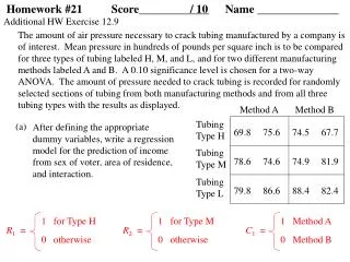
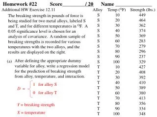
Homework #22 Score____________ / 20 Name ______________ Alloy Temp (OF) Strength (lbs.) S 10 449 S 20 464 S 30 362 S 40 374 S 50 369 S 60 283 S 70 279 S 80 296 S 90 237 S 100 329 T 10 427 T 20 408 T 30 392 T 40 410 T 50 389 T 60 380 T 70 413 T 80 356 T 90 334 T 100 348 Additional HW Exercise 12.11 (a) The breaking strength in pounds of force is being studied for two metal alloys, labeled S and T, and for different temperatures in OF. A 0.05 significance level is chosen for an analysis of covariance. A random sample of breaking strengths is recorded for various temperatures with the two alloys, and the results are displayed on the right. After defining the appropriate dummy variable for alloy, write a regression model for the prediction of breaking strength from alloy, temperature, and interaction. 1 for alloy S D = 0 for alloy T Y = breaking strength X = temperature
Y = 0 + 1D + 2X + 12DX + or E(Y) = 0 + 1D + 2X + 12DX Create an SPSS data file named metal containing three variables named alloy, temperature, and strength. Define codes for the variable alloy so that 1 (one) represents S, and 0 (zero) represents T. Store the data in this SPSS file by entering each temperature, breaking strength, and coded value for alloy. (b) (c) Use the Analyze >General Linear Model> Univariate options in SPSS to display the Univariate dialog box. Select the variable strength for the Dependent Variable slot, select the variable alloy for the Fixed Factor(s) section, and select the variable temperature for the Covariate(s) section. Click on the Model button to display the Univariate: Model dialogue box. Select the Custom option. Then, select the variable alloy from the list of variables in the Factors & Covariates section on the left, use the Build Term(s) arrow to enter this variable in the Model section on the right. Next, select the variable temperature from the list of variables in the Factors & Covariates section on the left, use the Build Term(s) arrow to enter this variable in the Model section on the right. Finally, select both variable names alloy and temperature before using the Build Term(s) arrow to enter the interaction variable (either alloy*temperature or temperature*alloy) in the Model section on the right. Click on the Continue button to return to the Univariate dialog box. continued next page
Additional HW Exercise 12.11(c) - continued Click on the Options button to display the Univariate: Options dialogue box. From the list in the Factor(s) and Factor Interactions section on the left, select OVERALL for the Display Means for section on the right, and select alloy for the Display Means for section on the right. Click on the Continue button to return to the Univariate dialog box. Click on the OK button, after which results are displayed in an SPSS output viewer window. Title the output to identify the homework exercise (Additional HW Exercise 12.11 - part (c)), your name, today’s date, and the course number (Math 214). Use the File > Print Preview options to see if any editing is needed before printing the output. Attach the printed copy to this assignment before submission.
(d) Summarize the results (Step 4) of the f test to see if there is sufficient evidence that the overall regression to predict breaking strength from alloy, temperature, and interaction is significant at the 0.05 level. Since f3,16 = have sufficient evidence to reject H0 . We conclude that 15.062 and f3,16;0.05 = 3.24, we the prediction of breaking strength from alloy, temperature, and interaction is significant (P < 0.01). OR (P < 0.001)
Additional HW Exercise 12.11 - continued (e) Summarize the results (Step 4) of the f test to see if there is sufficient evidence at the 0.05 level of a difference in mean breaking strength resulting from interaction between alloy and temperature. Based on the results of this f test, indicate why we should conclude that the regression to predict breaking strength from temperature is not parallel for alloys S and T. Since f1,16 = have sufficient evidence to reject H0 . We conclude that 5.369 and f1,16;0.05 = 4.49, we there is a difference in mean breaking strength resulting from interaction between alloy and temperature (0.025 < P < 0.05). OR (P = 0.034) Since we have rejected H0 , we should conclude that the regression to predict breaking strength from temperature is not parallel for alloys S and T.
Additional HW Exercise 12.11 - continued (g) (h) (i) Use the SPSS output from part (f) to write the least squares regression equation for predicting breaking strength from alloy, temperature, and interaction. strength = 432.667 + 23.867(D) – 0.854(temp) – 1.188(D)(temp) For each alloy, obtain a least squares regression equation for the prediction of breaking strength from temperature. For alloy S, D = 1 which implies strength = 432.667 + 23.867(1) – 0.854(temp) – 1.188(1)(temp)= 456.534 – 2.042(temp) For alloy T, D = 0 which implies strength = 432.667 + 23.867(0) – 0.854(temp) – 1.188(0)(temp)= 432.667 – 0.854(temp) Use SPSS to graph both least squares lines on a scatter plot by doing the following:
Additional HW Exercise 12.12 (a) The right-hand grip strength in pounds is being studied for right-handed males and females at different ages. A 0.05 significance level is chosen for an analysis of covariance. Right-hand grip strengths are recorded for random males and females of various ages, and the data is stored in the SPSS file named grip_compare. After looking at how sex is coded in the SPSS data file grip_compare, then define the appropriate dummy variable for sex, and write a regression model for the prediction of grip strength from sex, age, and interaction. Y = grip strength X = age 1 for female D = 0 for male Y = 0 + 1D + 2X + 12DX + or E(Y) = 0 + 1D + 2X + 12DX (b) After obtaining a copy of the SPSS file named grip_compare, note that the variable names are sex, age, and gripstrn. Use the SPSS instructions in part (c) of Additional HW Exercise 12.11 as a guide to obtain the same output for the data of this exercise that was obtained previously for the data of Additional HW Exercise 12.11.
Title the output to identify the homework exercise (Additional HW Exercise 12.12 - part (b)), your name, today’s date, and the course number (Math 214). Use the File > Print Preview options to see if any editing is needed before printing the output. Attach the printed copy to this assignment before submission. (c) Summarize the results (Step 4) of the f test to see if there is sufficient evidence that the overall regression to predict grip strength from sex, age, and interaction is significant at the 0.05 level. Since f3,18 = have sufficient evidence to reject H0 . We conclude that 120.707 and f3,18;0.05 = 3.16, we the prediction of grip strength from sex, age, and interaction is significant (P < 0.01). OR (P < 0.001)
Additional HW Exercise 12.12 - continued (d) Summarize the results (Step 4) of the f test to see if there is sufficient evidence at the 0.05 level of a difference in mean grip strength resulting from interaction between sex and age. Based on the results of this f test, explain why we should remove the interaction term from the model and conclude that the regression to predict grip strength from age is parallel for males and females. Since f1,18 = do not have sufficient evidence to reject H0 . We conclude that 1.157 and f1,18;0.05 = 4.41, we there is no difference in mean grip strength resulting from interaction between sex and age (0.10 < P). OR (P = 0.296) Since we have not rejected H0 , we should conclude that the regression to predict grip strength from age is parallel for males and females. (e) Use the Analyze >General Linear Model> Univariate options in SPSS to repeat part (b) without the interaction variable in the model.