Analysis of Tubing Pressure: Two-Way ANOVA and Regression Modeling
110 likes | 218 Vues
This homework exercise focuses on analyzing air pressure required to crack three tubing types (H, M, L) produced by two manufacturing methods (A, B). Through a two-way ANOVA at a significance level of 0.10, we evaluate the interaction between tubing type and manufacturing method on pressure values. We also build a regression model to predict pressure based on tubing type and method, initially including interactions and then eliminating them after testing for significance. Results are displayed using SPSS, elucidating the approach and findings of the statistical tests.

Analysis of Tubing Pressure: Two-Way ANOVA and Regression Modeling
E N D
Presentation Transcript
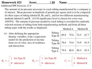
Homework #21 Score____________ / 10 Name ______________ Additional HW Exercise 12.9 (a) The amount of air pressure necessary to crack tubing manufactured by a company is of interest. Mean pressure in hundreds of pounds per square inch is to be compared for three types of tubing labeled H, M, and L, and for two different manufacturing methods labeled A and B. A 0.10 significance level is chosen for a two-way ANOVA. The amount of pressure needed to crack tubing is recorded for randomly selected sections of tubing from both manufacturing methods and from all three tubing types with the results as displayed. Method A Method B Tubing Type H After defining the appropriate dummy variables, write a regression model for the prediction of income from sex of voter, area of residence, and interaction. 69.8 75.6 74.5 67.7 Tubing Type M 78.6 74.6 74.9 81.9 Tubing Type L 79.8 86.6 88.4 82.4 1 for Type H R1 = 0 otherwise 1 for Type M R2 = 0 otherwise 1 Method A C1 = 0 Method B
Y = 0 + 1R1+ 2R2 + 3C1 + 11R1C1 + 21R2C1 + or E(Y) = 0 + 1R1+ 2R2 + 3C1 + 11R1C1 + 21R2C1 Create an SPSS data file named tubing containing three variables named type, method, and pressure. Define codes for the variable type so that 1 (one) represents H, 2 (two) represents M, and 3 (three) represents L. Define codes for the variable method so that 1 (one) represents A, and 2 (two) represents B. Store the data in this SPSS file by entering each pressure measurement together with the corresponding coded value for each tubing type and the coded value for each manufacturing method. (b)
Additional HW Exercise 12.9 - continued (c) Use the Analyze >General Linear Model> Univariate options in SPSS to display the Univariate dialog box. Select the variable pressure for the Dependent Variable slot, and select the variables type and method for the Fixed Factor(s) section. Click on the Options button to display the Univariate: Options dialogue box. From the list in the Factor(s) and Factor Interactions section on the left, select type*method for the Display Means for section on the right. Click on the Continue button to return to the Univariate dialog box. Click on the OK button, after which results are displayed in an SPSS output viewer window. Title the output to identify the homework exercise (Additional HW Exercise 12.9 - part (c)), your name, today’s date, and the course number (Math 214). Use the File > Print Preview options to see if any editing is needed before printing the output. Attach the printed copy to this assignment before submission. (d) Summarize the results (Step 4) of the f test to see if there is sufficient evidence that the overall regression to predict pressure from tubing type, manufacturing method, and interaction is significant at the 0.10 level.
Since f5,6 = have sufficient evidence to reject H0 . We conclude that 3.372 and f5,6;0.10 = 3.11, we the prediction of pressure from tubing type, manufacturing method, and interaction is significant (0.05 < P < 0.10). OR (P < 0.086) (e) Summarize the results (Step 4) of the f test to see if there is sufficient evidence at the 0.10 level of a difference in mean pressure resulting from interaction between tubing type and manufacturing method. Based on the results of this f test, explain why the next step in the two-way ANOVA is to eliminate interaction from the model. Since f2,6 = do not have sufficient evidence to reject H0 . We conclude that 0.230 and f2,6;0.10 = 3.46, we there is no difference in mean pressure resulting from interaction between tubing type and manufacturing method (0.10 < P). Since we have not rejected H0 and concluded that no interaction exists, we eliminate interaction from the model. OR (P = 0.801)
Additional HW Exercise 12.9 - continued (f) (g) Using the dummy variables defined in part (a), write a regression model for the prediction of pressure from tubing type and manufacturing method with no interaction. Y = 0 + 1R1+ 2R2 + 3C1 + or E(Y) = 0 + 1R1+ 2R2 + 3C1 Use the Analyze >General Linear Model> Univariate options in SPSS to display the Univariate dialog box. Select the variable pressure for the Dependent Variable slot, and select the variables type and method for the Fixed Factor(s) section. Click on the Model button to display the Univariate: Model dialogue box. Select the Custom option. Then, from the list of variables in the Factors & Covariates section on the left, use the Build Term(s) arrow to select the variable type for the Model section on the right, and to select the variable method for the Model section. Click on the Continue button to return to the Univariate dialog box. Click on the Options button to display the Univariate: Options dialogue box. From the list in the Factor(s) and Factor Interactions section on the left, select type for the Display Means for section on the right, and also select method for the Display Means for section. Click on the Continue button to return to the Univariate dialog box.
Click on the Post Hoc button to display the Univariate: Post Hoc Multiple Comparisons for Observed Means dialogue box. From the list of variables in the Factor(s) section on the left, select the variable type for the Post Hoc Tests for section on the right. Then, select the Tukey option. (There is no need to select method for multiple comparison, since this variable only has two categories!) Click on the Continue button to return to the Univariate dialogue box. Click on the OK button, after which results are displayed in an SPSS output viewer window. Title the output to identify the homework exercise (Additional HW Exercise 12.9 - part (g)), your name, today’s date, and the course number (Math 214). Use the File > Print Preview options to see if any editing is needed before printing the output. Attach the printed copy to this assignment before submission.
Additional HW Exercise 12.9 - continued (h) Summarize the results (Step 4) of the f test to see if there is sufficient evidence that the overall regression to predict pressure from tubing type and manufacturing method (with no interaction) is significant at the 0.10 level. Since f3,8 = have sufficient evidence to reject H0 . We conclude that 6.769 and f3,8;0.05 = 2.92, we the prediction of pressure from tubing type and manufacturing method (with no interaction) is significant (0.01 < P < 0.025). OR (P = 0.014) (i) Summarize the results (Step 4) of the f test to see if there is sufficient evidence at the 0.10 level of a difference in mean pressure resulting from tubing type.
Since f2,8 = have sufficient evidence to reject H0 . We conclude that 10.091 and f2,8;0.10 = 3.11, we the there is a difference in mean pressure resulting from tubing type (P < 0.01). OR (P = 0.006) (j) Summarize the results (Step 4) of the f test to see if there is sufficient evidence at the 0.10 level of a difference in mean pressure resulting from manufacturing method. Since f1,8 = do not have sufficient evidence to reject H0 . We conclude that 0.126 and f1,8;0.10 = 3.46, we the there is a difference in mean pressure resulting from manufacturing method (0.10 < P). OR (P = 0.732)
Additional HW Exercise 12.9 - continued (k) Based on the results in parts (i) and (j), decide whether or not a multiple comparison method is necessary. If no, then explain why not; if yes, then use Tukey’s HSD multiple comparison method with = 0.10. A significant difference in mean pressure resulting from tubing typewas found, implying that multiple comparison is necessary. We can identify significant differences from the results of Tukey’s HSD on the SPSS output. With = 0.10, we conclude that mean pressure is higher for tubing type L than for tubing type H, and that mean pressure is higher for tubing type L than for tubing typeM. A significant difference in mean pressure resulting from manufacturing methodwas not found, so no further analysis involving manufacturing method is necessary.
(l) Describe below what would be an appropriate graphical display for the results in part (k), and explain why. Then, use SPSS to create this graphical display. Title the output to identify the homework exercise (Additional HW Exercise 12.9 - part (l)), your name, today’s date, and the course number (Math 214). Since the quantitative variable pressure is being compared for the three tubing types and also for the two manufacturing methods, contiguous box plots are appropriate in each case. However. we may choose not to display box plots for the two manufacturing methods, since no statistically significant difference was found.
Additional HW Exercise 12.10 (a) A two-way analysis of variance is used to study the mean lifetime in hours for three brands of light bulbs, Brite, Softlite, and Nodark, and for two levels of brightness, 50 watt and 100 watt. A 0.05 significance level is chosen for hypothesis testing. With each combination of brand and brightness, lifetimes are recorded for 4 bulbs. Complete the following two-way ANOVA table: 5 1496 299.2 3.12 0.01 < P < 0.05 2 112 56 0.58 0.10 < P 1 216 216 2.25 0.10 < P 2 1168 584 6.08 P < 0.01 18 1728 96 23 3224