Statistical Methods (Lectures 2.1, 2.2)
1.3k likes | 1.5k Vues
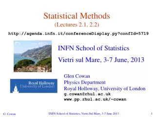
Statistical Methods (Lectures 2.1, 2.2). http://agenda.infn.it/conferenceDisplay.py?confId=5719. INFN School of Statistics Vietri sul Mare, 3-7 June, 2013. Glen Cowan Physics Department Royal Holloway, University of London g.cowan@rhul.ac.uk www.pp.rhul.ac.uk/~cowan. Rough outline.

Statistical Methods (Lectures 2.1, 2.2)
E N D
Presentation Transcript
Statistical Methods(Lectures 2.1, 2.2) http://agenda.infn.it/conferenceDisplay.py?confId=5719 INFN School of Statistics Vietri sul Mare, 3-7 June, 2013 Glen Cowan Physics Department Royal Holloway, University of London g.cowan@rhul.ac.uk www.pp.rhul.ac.uk/~cowan INFN School of Statistics, Vietri Sul Mare, 3-7 June 2013
Rough outline I. Basic ideas of parameter estimation II. The method of Maximum Likelihood (ML) Variance of ML estimators Extended ML III. Method of Least Squares (LS) IV. Bayesian parameter estimation V. Goodness of fit from the likelihood ratio VI. Examples of frequentist and Bayesian approaches INFN School of Statistics, Vietri Sul Mare, 3-7 June 2013
Parameter estimation The parameters of a pdf are constants that characterize its shape, e.g. r.v. parameter Suppose we have a sample of observed values: We want to find some function of the data to estimate the parameter(s): ← estimator written with a hat Sometimes we say ‘estimator’ for the function of x1, ..., xn; ‘estimate’ for the value of the estimator with a particular data set. INFN School of Statistics, Vietri Sul Mare, 3-7 June 2013
Properties of estimators If we were to repeat the entire measurement, the estimates from each would follow a pdf: best large variance biased We want small (or zero) bias (systematic error): → average of repeated measurements should tend to true value. And we want a small variance (statistical error): →small bias & variance arein general conflicting criteria INFN School of Statistics, Vietri Sul Mare, 3-7 June 2013
An estimator for the mean (expectation value) Parameter: (‘sample mean’) Estimator: We find: INFN School of Statistics, Vietri Sul Mare, 3-7 June 2013
An estimator for the variance Parameter: (‘sample variance’) Estimator: We find: (factor of n-1 makes this so) where INFN School of Statistics, Vietri Sul Mare, 3-7 June 2013
The likelihood function Suppose the entire result of an experiment (set of measurements) is a collection of numbers x, and suppose the joint pdf for the data x is a function that depends on a set of parameters q: Now evaluate this function with the data obtained and regard it as a function of the parameter(s). This is the likelihood function: (x constant) INFN School of Statistics, Vietri Sul Mare, 3-7 June 2013
The likelihood function for i.i.d.*. data * i.i.d. = independent and identically distributed Consider n independent observations of x: x1, ..., xn, where x follows f (x; q). The joint pdf for the whole data sample is: In this case the likelihood function is (xi constant) INFN School of Statistics, Vietri Sul Mare, 3-7 June 2013
Maximum likelihood estimators If the hypothesized q is close to the true value, then we expect a high probability to get data like that which we actually found. So we define the maximum likelihood (ML) estimator(s) to be the parameter value(s) for which the likelihood is maximum. ML estimators not guaranteed to have any ‘optimal’ properties, (but in practice they’re very good). INFN School of Statistics, Vietri Sul Mare, 3-7 June 2013
ML example: parameter of exponential pdf Consider exponential pdf, and suppose we have i.i.d. data, The likelihood function is The value of t for which L(t) is maximum also gives the maximum value of its logarithm (the log-likelihood function): INFN School of Statistics, Vietri Sul Mare, 3-7 June 2013
ML example: parameter of exponential pdf (2) Find its maximum by setting → Monte Carlo test: generate 50 values using t = 1: We find the ML estimate: INFN School of Statistics, Vietri Sul Mare, 3-7 June 2013
Functions of ML estimators Suppose we had written the exponential pdf as i.e., we use l = 1/t. What is the ML estimator for l? For a function a(q) of a parameter q, it doesn’t matter whether we express L as a function of a or q. The ML estimator of a function a(q) is simply So for the decay constant we have is biased, even though is unbiased. Caveat: Can show (bias →0 for n →∞) INFN School of Statistics, Vietri Sul Mare, 3-7 June 2013
Example of ML: parameters of Gaussian pdf Consider independent x1, ..., xn, with xi ~ Gaussian (m,s2) The log-likelihood function is INFN School of Statistics, Vietri Sul Mare, 3-7 June 2013
Example of ML: parameters of Gaussian pdf (2) Set derivatives with respect to m, s2 to zero and solve, We already know that the estimator for m is unbiased. But we find, however, so ML estimator for s2 has a bias, but b→0 for n→∞. Recall, however, that is an unbiased estimator for s2. INFN School of Statistics, Vietri Sul Mare, 3-7 June 2013
Variance of estimators: Monte Carlo method Having estimated our parameter we now need to report its ‘statistical error’, i.e., how widely distributed would estimates be if we were to repeat the entire measurement many times. One way to do this would be to simulate the entire experiment many times with a Monte Carlo program (use ML estimate for MC). For exponential example, from sample variance of estimates we find: Note distribution of estimates is roughly Gaussian − (almost) always true for ML in large sample limit. INFN School of Statistics, Vietri Sul Mare, 3-7 June 2013
Variance of estimators from information inequality The information inequality (RCF) sets a lower bound on the variance of any estimator (not only ML): Minimum Variance Bound (MVB) Often the bias b is small, and equality either holds exactly or is a good approximation (e.g. large data sample limit). Then, Estimate this using the 2nd derivative of ln L at its maximum: INFN School of Statistics, Vietri Sul Mare, 3-7 June 2013
Variance of estimators: graphical method Expand ln L (q) about its maximum: First term is ln Lmax, second term is zero, for third term use information inequality (assume equality): i.e., → to get , change q away from until ln L decreases by 1/2. INFN School of Statistics, Vietri Sul Mare, 3-7 June 2013
Example of variance by graphical method ML example with exponential: Not quite parabolic ln L since finite sample size (n = 50). INFN School of Statistics, Vietri Sul Mare, 3-7 June 2013
Information inequality for n parameters Suppose we have estimated n parameters The (inverse) minimum variance bound is given by the Fisher information matrix: The information inequality then states that V-I-1 is a positive semi-definite matrix, where Therefore Often use I-1 as an approximation for covariance matrix, estimate using e.g. matrix of 2nd derivatives at maximum of L. INFN School of Statistics, Vietri Sul Mare, 3-7 June 2013
Example of ML with 2 parameters Consider a scattering angle distribution with x = cos q, or if xmin < x < xmax, need always to normalize so that Example: a = 0.5, b = 0.5, xmin = -0.95, xmax = 0.95, generate n = 2000 events with Monte Carlo. INFN School of Statistics, Vietri Sul Mare, 3-7 June 2013
Example of ML with 2 parameters: fit result Finding maximum of ln L(a, b) numerically (MINUIT) gives N.B.No binning of data for fit, but can compare to histogram for goodness-of-fit (e.g. ‘visual’ or c2). (MINUIT routine HESSE) (Co)variances from INFN School of Statistics, Vietri Sul Mare, 3-7 June 2013
Two-parameter fit: MC study Repeat ML fit with 500 experiments, all with n = 2000 events: Estimates average to ~ true values; (Co)variances close to previous estimates; marginal pdfs approximately Gaussian. INFN School of Statistics, Vietri Sul Mare, 3-7 June 2013
The ln Lmax- 1/2 contour For large n, ln L takes on quadratic form near maximum: is an ellipse: The contour INFN School of Statistics, Vietri Sul Mare, 3-7 June 2013
(Co)variances from ln L contour The a, b plane for the first MC data set → Tangent lines to contours give standard deviations. → Angle of ellipse f related to correlation: Correlations between estimators result in an increase in their standard deviations (statistical errors). INFN School of Statistics, Vietri Sul Mare, 3-7 June 2013
Extended ML Sometimes regard n not as fixed, but as a Poisson r.v., mean n. Result of experiment defined as: n, x1, ..., xn. The (extended) likelihood function is: Suppose theory gives n = n(q), then the log-likelihood is where C represents terms not depending on q. INFN School of Statistics, Vietri Sul Mare, 3-7 June 2013
Extended ML (2) Example: expected number of events where the total cross section s(q) is predicted as a function of the parameters of a theory, as is the distribution of a variable x. Extended ML uses more info → smaller errors for Important e.g. for anomalous couplings in e+e-→ W+W- If n does not depend on q but remains a free parameter, extended ML gives: INFN School of Statistics, Vietri Sul Mare, 3-7 June 2013
Extended ML example Consider two types of events (e.g., signal and background) each of which predict a given pdf for the variable x: fs(x) and fb(x). We observe a mixture of the two event types, signal fraction = q, expected total number = n, observed total number = n. goal is to estimate ms, mb. Let → INFN School of Statistics, Vietri Sul Mare, 3-7 June 2013
Extended ML example (2) Monte Carlo example with combination of exponential and Gaussian: Maximize log-likelihood in terms of ms and mb: Here errors reflect total Poisson fluctuation as well as that in proportion of signal/background. INFN School of Statistics, Vietri Sul Mare, 3-7 June 2013
Extended ML example: an unphysical estimate A downwards fluctuation of data in the peak region can lead to even fewer events than what would be obtained from background alone. Estimate for ms here pushed negative (unphysical). We can let this happen as long as the (total) pdf stays positive everywhere. INFN School of Statistics, Vietri Sul Mare, 3-7 June 2013
Unphysical estimators (2) Here the unphysical estimator is unbiased and should nevertheless be reported, since average of a large number of unbiased estimates converges to the true value (cf. PDG). Repeat entire MC experiment many times, allow unphysical estimates: INFN School of Statistics, Vietri Sul Mare, 3-7 June 2013
ML with binned data Often put data into a histogram: Hypothesis is where If we model the data as multinomial (ntot constant), then the log-likelihood function is: INFN School of Statistics, Vietri Sul Mare, 3-7 June 2013
ML example with binned data Previous example with exponential, now put data into histogram: Limit of zero bin width → usual unbinned ML. If ni treated as Poisson, we get extended log-likelihood: INFN School of Statistics, Vietri Sul Mare, 3-7 June 2013
Relationship between ML and Bayesian estimators In Bayesian statistics, both q and x are random variables: Recall the Bayesian method: Use subjective probability for hypotheses (q); before experiment, knowledge summarized by prior pdf p(q); use Bayes’ theorem to update prior in light of data: Posterior pdf (conditional pdf for q given x) INFN School of Statistics, Vietri Sul Mare, 3-7 June 2013
ML and Bayesian estimators (2) Purist Bayesian: p(q | x) contains all knowledge about q. Pragmatist Bayesian: p(q | x) could be a complicated function, →summarize using an estimator Take mode of p(q | x) , (could also use e.g. expectation value) What do we use for p(q)? No golden rule (subjective!), often represent ‘prior ignorance’ by p(q) = constant, in which case But... we could have used a different parameter, e.g., l = 1/q, and if prior pq(q) is constant, then pl(l) is not! ‘Complete prior ignorance’ is not well defined. INFN School of Statistics, Vietri Sul Mare, 3-7 June 2013
Priors from formal rules Because of difficulties in encoding a vague degree of belief in a prior, one often attempts to derive the prior from formal rules, e.g., to satisfy certain invariance principles or to provide maximum information gain for a certain set of measurements. Often called “objective priors” Form basis of Objective Bayesian Statistics The priors do not reflect a degree of belief (but might represent possible extreme cases). In a Subjective Bayesian analysis, using objective priors can be an important part of the sensitivity analysis. INFN School of Statistics, Vietri Sul Mare, 3-7 June 2013
Priors from formal rules (cont.) In Objective Bayesian analysis, can use the intervals in a frequentist way, i.e., regard Bayes’ theorem as a recipe to produce an interval with certain coverage properties. For a review see: Formal priors have not been widely used in HEP, but there is recent interest in this direction; see e.g. L. Demortier, S. Jain and H. Prosper, Reference priors for high energy physics, arxiv:1002.1111 (Feb 2010) INFN School of Statistics, Vietri Sul Mare, 3-7 June 2013
Jeffreys’ prior According to Jeffreys’rule, take prior according to where is the Fisher information matrix. One can show that this leads to inference that is invariant under a transformation of parameters. For a Gaussian mean, the Jeffreys’ prior is constant; for a Poisson mean m it is proportional to 1/√m. INFN School of Statistics, Vietri Sul Mare, 3-7 June 2013
Jeffreys’ prior for Poisson mean Suppose n ~ Poisson(m). To find the Jeffreys’ prior for m, So e.g. for m = s + b, this means the prior p(s) ~ 1/√(s + b), which depends on b. But this is not designed as a degree of belief about s. INFN School of Statistics, Vietri Sul Mare, 3-7 June 2013
The method of least squares Suppose we measure N values, y1, ..., yN, assumed to be independent Gaussian r.v.s with Assume known values of the control variable x1, ..., xN and known variances We want to estimate θ, i.e., fit the curve to the data points. The likelihood function is INFN School of Statistics, Vietri Sul Mare, 3-7 June 2013
The method of least squares (2) The log-likelihood function is therefore So maximizing the likelihood is equivalent to minimizing Minimum defines the least squares (LS) estimator Very often measurement errors are ~Gaussian and so ML and LS are essentially the same. Often minimize χ2 numerically (e.g. program MINUIT). INFN School of Statistics, Vietri Sul Mare, 3-7 June 2013
LS with correlated measurements If the yi follow a multivariate Gaussian, covariance matrix V, Then maximizing the likelihood is equivalent to minimizing INFN School of Statistics, Vietri Sul Mare, 3-7 June 2013
Example of least squares fit Fit a polynomial of order p: INFN School of Statistics, Vietri Sul Mare, 3-7 June 2013
Variance of LS estimators In most cases of interest we obtain the variance in a manner similar to ML. E.g. for data ~ Gaussian we have and so 1.0 or for the graphical method we take the values of θ where INFN School of Statistics, Vietri Sul Mare, 3-7 June 2013
Two-parameter LS fit INFN School of Statistics, Vietri Sul Mare, 3-7 June 2013
Goodness-of-fit with least squares The value of the χ2 at its minimum is a measure of the level of agreement between the data and fitted curve: It can therefore be employed as a goodness-of-fit statistic to test the hypothesized functional form λ(x; θ). We can show that if the hypothesis is correct, then the statistic t = χ2min follows the chi-square pdf, where the number of degrees of freedom is nd = number of data points - number of fitted parameters INFN School of Statistics, Vietri Sul Mare, 3-7 June 2013
Goodness-of-fit with least squares (2) The chi-square pdf has an expectation value equal to the number of degrees of freedom, so if χ2min≈ nd the fit is ‘good’. More generally, find the p-value: This is the probability of obtaining a χ2min as high as the one we got, or higher, if the hypothesis is correct. E.g. for the previous example with 1st order polynomial (line), whereas for the 0th order polynomial (horizontal line), INFN School of Statistics, Vietri Sul Mare, 3-7 June 2013
Goodness-of-fit vs. statistical errors INFN School of Statistics, Vietri Sul Mare, 3-7 June 2013
Goodness-of-fit vs. stat. errors (2) INFN School of Statistics, Vietri Sul Mare, 3-7 June 2013
LS with binned data INFN School of Statistics, Vietri Sul Mare, 3-7 June 2013
LS with binned data (2) INFN School of Statistics, Vietri Sul Mare, 3-7 June 2013