Statistical methods of data analysis
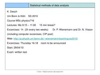
Statistical methods of data analysis. K. Desch Uni Bonn & Köln SS 2010 Course MSc physics716 Lectures: Mo 9:15 – 11:00 15 min break? Excercises: 1h (2h every two weeks) Dr. P. Wienemann and Dr. N. Vlasov (including computer excercises, CIP pool)

Statistical methods of data analysis
E N D
Presentation Transcript
Statistical methods of data analysis K. Desch Uni Bonn & Köln SS 2010 Course MSc physics716 Lectures: Mo 9:15 – 11:00 15 min break? Excercises: 1h (2h every two weeks) Dr. P. Wienemann and Dr. N. Vlasov (including computer excercises, CIP pool) Web: http://pi.physik.uni-bonn.de/~wienemann/teaching/ss2010/ Excercises: Thursday 16-18 room to be announced Start: 29/04/10 Exam: written test K. Desch – Statistical methods of data analysis SS10
Literature and resources Books: G. Cowan: Statistical Data Analysis, Oxford University Press (1998), 35€ R. J. Barlow, Statistics: A Guide to the Use of Statistical Methods in the Physical Sciences, John Wiley (1993), 39€ S. Brandt: Datenanalyse, Spektrum Akademischer Verlag (1999), 26€ Computer programs, tools: root http://root.cern.ch data analysis RooFit http://roofit.sourceforge.net/ fitting RooStats https://twiki.cern.ch/twiki/bin/view/RooStats/WebHome statistical tests… K. Desch – Statistical methods of data analysis SS10
Contents • Introduction • Probablity functions • Monte Carlo method • Testing hypotheses • Estimation • Maximum Likelihood • Method of least squares • Statistical errors, confidence intervals, limits • … K. Desch – Statistical methods of data analysis SS10
1. Introduction 1.1. Statistics in physics • Describe data sets (e.g. sets of measurements) with few numbers • (mean, variance, …) = descriptive statistics • Randomness in statististical physics • Describe the properties of large ensembles and derive laws of nature • for these ensembles (not for the individual particles) • (note: classical physics is deterministic – but many unknown boundary • conditions – “seemingly” random) • Randomness in quantum mechanics • probability interpretation of wave function • Describe measurement errors (uncertaintiy) • statististical errors: “known” (estimable, assessable) probability distribution • systematic errors: “unknown” (or no) probability distribution K. Desch – Statistical methods of data analysis SS10
1. Introduction 1.1. Statistics in physics • Hypothesis testing • Compare data with a theoretical model • Determine (“fit”) the parameters of a theoretical model and theirerrors • Note: • “Error” (= “uncertainty”) in physics: • True value lies within the error interval with a certain probability • (c.f. “tolerances” in engineering) K. Desch – Statistical methods of data analysis SS10
1. Introduction 1.1. Statistics in physics Measurement = Compare measured value to a scaleMeasurement = Estimate a parameter of a theoretical model from data Example: measurement of the mass of the W-boson K. Desch – Statistical methods of data analysis SS10
1. Introduction 1.1. Statistics in physics Testing hypotheses Higgs or no Higgs? exclusion limits confidence levels K. Desch – Statistical methods of data analysis SS10
1. Introduction 1.1. Statistics in physics Statistical numerical methods: e.g. integration Also works in N dimensionens (where classical methods fail…) K. Desch – Statistical methods of data analysis SS10
1. Introduction 1.1. Statistics in physics Simulation of particle/nuclear physics experiments Variety of statistical processes matrix element particle transport detector response in detail… K. Desch – Statistical methods of data analysis SS10
1. Introduction 1.2. Randomness and Probability Christian Huygens De Ratiociniis in Ludo Aleae(1657) 14 theses about probability theory K. Desch – Statistical methods of data analysis SS10
1. Introduction 1.2. Randomness and Probability Andrei Kolmogorov (1903-1987) Axiome zur mathematischenDefinition von Wahrscheinlichkeit Heidelberg 1933 K. Desch – Statistical methods of data analysis SS10
1. Introduction 1.3. Kolmogorov Axioms • Mathematical definition of probability • (no meaning/interpretation what probability actually means, • good: conclusions following from Kolmogorov-Axioms are • independent of the interpretation of probability) • Set S of “samples” (“events”) (sample space) • Assign a real number P(A) to each subset A of S • P(A) := probability of A • with the following properties: • P(A) 0 for each subset A of S • P(S) = 1 • P(AB) = P(A) + P(B) • for disjoint subsets A and B (AB=Ø) K. Desch – Statistical methods of data analysis SS10
1. Introduction 1.3. Kolmogorov Axioms Implications (w/o proof) P(Ø) = 0 0 P(A) 1 AB P(A) P(B) P(AB) = P(A) + P(B) – P(AB) Complement of A: A and B are called statistically independent (or uncorrelated) if P(AB) = P(A)P(B) If an event belongs to A nothing is implied about its belonging to B Important concept! K. Desch – Statistical methods of data analysis SS10
1. Introduction 1.3. Kolmogorov Axioms Example 1 (uncorrelated): S = all students of Bonn university A = all male students of Bonn university B = all students whose birthday is between Jan 1st and April 30th A and B are (presumably) uncorrelated, therefore P(AB) = P(A)P(B) Example 2 (correlated): S = all people living in germany A = all people living in germany under the age of 12 years B = all people living in germany shorter than 150 cm A and B are (strongly) positively correlated, i.e. P(AB) > P(A)*P(B) K. Desch – Statistical methods of data analysis SS10
1. Introduction 1.3. Kolmogorov Axioms Example 3: Muon decay at rest e K. Desch – Statistical methods of data analysis SS10
1. Introduction 1.3. Kolmogorov Axioms Example 3: Muon decay in flight e K. Desch – Statistical methods of data analysis SS10
1. Introduction 1.3. Kolmogorov Axioms Example 4: Measurement of the ratio Identification of b-quarks through secondary vertex Needed: efficiency to “tag” a b-jet P(b) Determine from “double tags” assuming works only if probability to tag either jet are uncorrelated! K. Desch – Statistical methods of data analysis SS10
1. Introduction 1.3. Kolmogorov Axioms 1994 K. Desch – Statistical methods of data analysis SS10
1. Introduction 1.3. Kolmogorov Axioms today K. Desch – Statistical methods of data analysis SS10
1. Introduction 1.4. Conditional probability and Bayes theorem Probability for A given B: A B S Probability for B given A: Bayes theorem: Split S in disjoint subsets Ai i.e. then combined with Bayes theorem: for any subset A, e.g. for one of the Ai K. Desch – Statistical methods of data analysis SS10
1. Introduction 1.4. Conditional probability and Bayes theorem Example: disease known to be carried by 0.2% of the population. Prior probability: a rather reliable blood test for the disease yields and a small probability for a false positive result What is the probability to have the disease if you are tested positive? K. Desch – Statistical methods of data analysis SS10
1. Introduction 1.4. Conditional probability and Bayes theorem • small probability of having the disease even if tested positive by a highly • reliable test K. Desch – Statistical methods of data analysis SS10
1. Introduction 1.5. Interpretation of “probability” • 1.5.1. Probability as a relative frequency: “Frequentist interpretation” • elements of S are the possible outcomes of a measurement • assume measurement can be (at least hypothetically) repeated • Subset A: occurrence of of any of the outcomes in the subset A • Define probability • This the natural interpretation of probability in • quantum mechanics • statistical mechanics • consistent with Kolmogorov axioms • can never be determined perfectly ( estimation) Simon Laplace 1749-1827 K. Desch – Statistical methods of data analysis SS10
1. Introduction 1.5. Interpretation of “probability” • 1.5.2. Subjective („Bayesian“) probability „Bayes interpretation“ • elements of sample space S are „hypotheses“ or „propositions“ • (i.e. statements which are true or false) • Interpretation of probability • P(A) = degree of belief that the hypothesis A is true • Bayes statistics: • A = hypothesis that a theory is true • B = hypothesis that experiment yields a certain result • Bayes theorem: • Problematic interpretation of P(theory) („a priori“ probability, „prior probability“) • No fundamental rule how to define a prior – but once it is done, no need to • estimate the „posterior“ probability, it can be calculated Rev. Thomas Bayes 1702-1761 K. Desch – Statistical methods of data analysis SS10
1. Introduction 1.5. Interpretation of “probability” In the following we will mainly work in the „frequentist“ picture There are certain limits within which frequentist and Bayesian statistics will yield the same result We will discuss Bayesian statistics in the context of the principle of maximum likelihood and when setting confidence limits K. Desch – Statistical methods of data analysis SS10
2. Probability 2.1. Probability density functions Simplest case: measurement can only take discrete values xi (e.g. couting experiment, xi = number of counts) probability to measure xi : P(xi) =: fi Often the result of a measurement is a continous quantitiy x Probability to obtain exactly x is zero Better: probability to obtain a measurement in the interval [x+dx] P([x+dx]) =: f(x) dx f(x) = probability densitiy function (p.d.f.) with Integration of f(x) yields a probability: Cumulative Distribution: yields the probability to obtain a measurement smaller than x K. Desch – Statistical methods of data analysis SS10
2. Probability 2.1. Probabilitydensityfunctions Probability that measurement lies in the interval [a,b] is F(b)-F(a) For discrete random variables Example for a p.d.f. and its cumulative distribution: K. Desch – Statistical methods of data analysis SS10
2. Probability 2.2. Characterizing p.d.f.´s Quantile: Median: (50%-value) Most probable value: maximum of f(x) Mean value: discrete distribution: K. Desch – Statistical methods of data analysis SS10
2. Probability 2.2. Characterizing p.d.f.´s Histogram: frequency distribution of events Normalized to area = 1: bin contents/bin width ~ f(x) (in the limit bin width 0) K. Desch – Statistical methods of data analysis SS10
2. Probability 2.2. Characterizing p.d.f.´s Expectation value of a function a(x): For a(x) = x one yields the mean value Expectation values of powers of x are called moments of a p.d.f. algebraic moments: central moments: K. Desch – Statistical methods of data analysis SS10
2. Probability 2.2. Characterizing p.d.f.´s A measure for the width of a distribution (p.d.f.) is the variance: The variance is the second central moment von f(x), i.e. its mean square deviation from the mean value. standard deviation: (same units as x, ) From linearity of expectation values follows (will be useful later for estimating the variance of discrete p.d.f.´s) K. Desch – Statistical methods of data analysis SS10
2. Probability 2.2. Characterizing p.d.f.´s Higher moments: Skewness: Measure for the asymmetry of a distribution Kurtosis: Measures importance of “tails” of a distribution Larger tails than Gaussian: > 0 Smaller tails than Gaussian: < 0 K. Desch – Statistical methods of data analysis SS10

