Statistical Methods for Data Analysis hypothesis testing
Statistical Methods for Data Analysis hypothesis testing. Luca Lista INFN Napoli. Contents. Hypothesis testing Neyman-Pearson lemma and likelihood ratio Multivariate analysis (elements) Chi-square fits and goodness-of-fit Confidence intervals Feldman-Cousins ordering. Hypothesis testing.

Statistical Methods for Data Analysis hypothesis testing
E N D
Presentation Transcript
Statistical Methodsfor Data Analysishypothesis testing Luca Lista INFN Napoli
Contents • Hypothesis testing • Neyman-Pearson lemma and likelihood ratio • Multivariate analysis (elements) • Chi-square fits and goodness-of-fit • Confidence intervals • Feldman-Cousins ordering Statistical methods in LHC data analysis
Hypothesis testing • The problem from the point of view of a physicist: • A data sample is characterized by n variables, (x1, …, xn), with different distributions for two cases possible process: signal, and background • Given a measurement (= event) of the n variables having discriminating power, identify (discriminate) the event as coming from signal or background • Clearly, the identification sometimes gives the correct answer, sometimes gives the wrong answer • Property of discriminator: • Selection efficiency: probability to correctly identify signal events • Misidentification probability: probability to misidentify as a background event • Purity: fraction of signal in a positively identified sample • Depends on the signal and background composition! It is not a property of the discriminator only • Fake rate: fraction of background in a positively identified sample, = 1- Purity Statistical methods in LHC data analysis
Terminology for statisticians • Statisticians’ terminology is usually less natural for physics applications than previous slide, but is intended for a more general applicability • H0 = null hypothesis • E.g.: a sample contains only background; a particle is a pion; etc. • H1 = alternative hypothesis • E.g.: a sample contains background + signal; or a particle is a muon; etc. • = significance level: probability to reject H1 if true (error of first kind), i.e. assuming H1 • = 1 – selection efficiency • = probability to reject H0 if true (error of second kind), i.e. assuming H0 • = misidentification probability Statistical methods in LHC data analysis
Cut analysis • Cut on one (or more) variables: • If xxcut signal • Else, if xxcut background Efficiency (1-) Mis-id probability() xcut x Statistical methods in LHC data analysis
Variations on cut analyses • Cut on multiple variables • AND/OR of single cuts • Multi-dimensional cuts: • Linear cuts • Piece-wise linear cuts • Non-linear combinations • At some point, hard to find optimal cut values, or too many cuts required • How to determine the cuts, looking at control samples? • Control samples could be MC, or selected data decays • Note: cut selection must be done a-priori, before looking at data, to avoid biases! Statistical methods in LHC data analysis
Efficiency vs mis-id • Varying the cut both the efficiency and mis-id change 1 Efficiency xcut 0 0 1 Mis-id Statistical methods in LHC data analysis
Straight cuts or something else? • Straight cuts may not be optimal in all cases Statistical methods in LHC data analysis
Likelihood ratio discriminator • We make the ratio of likelihoods defined in the two hypotheses: • Q may also depend on a number of unknown parameters (1,…,N) • Best discriminator, if the multi-dimensional likelihood is perfectly known (Neyman-Pearson lemma) • Great effort in getting the correct ratio • E.g.: Matrix Element Tecnhniques for top mass and single-top at Tevatron Statistical methods in LHC data analysis
Neyman-Pearson lemma • Fixing the signal efficiency (1− ), a selection based on the likelihood ratio gives the lowest possible mis-id probability (): (x) = L(x|H1) / L(x|H0) > k • If we can’t use the likelihood ratio, we can choose other discriminators, or “test statistics”: • A test statistic is any function of x (like (x)) that allows to discriminate the two hypotheses • Neural networks, boosted decision trees are example of discriminators that may closely approximate the performances of Neyman-Pearson limit Statistical methods in LHC data analysis
Likelihood factorization • We make the ratio of likelihoods defined in the two hypotheses assuming PDF factorized as product of 1-D PDF: • Approximate in case of non perfectly factorized PDF • E.g.: correlation • A rotation or other judicious transformations in the variables’ space may be used to remove the correlation • Sometimes even different for s and b hypotheses If PDF can be factorized into independent components Statistical methods in LHC data analysis
Building projective PDF’s • PDF’s for likelihood discriminator • If not uncorrelated, need to find uncorrelated variables first, otherwise plain PDF product is suboptimal Statistical methods in LHC data analysis
Likelihood ratio output • Good separation achieved in this case TMVA L > 0.5 Statistical methods in LHC data analysis
Fisher discriminator • Combine a number of variables into a single discriminator • Equivalent to project the distribution along a line • Use the linear combination of inputs that maximizes the distance of the means of the two classes while minimizing the variancewithin each class: • The maximization problem can be solved with linear algebra Sir Ronald Aylmer Fisher (1890-1962) Statistical methods in LHC data analysis
Rewriting Fisher discriminant • m1, m2 are the two samples’ average vectors • 1, 2 are the two samples’ covariance matrices • Transform with linear vector of coefficients w • w is normal to the discriminator hyperplane “between classes scatter matrix” “within classes scatter matrix” Statistical methods in LHC data analysis
Maximizing the Fisher discriminant • Either compute derivatives w.r.t. wi • Equivalent to solve the eigenvalues problem: Statistical methods in LHC data analysis
Fisher in the previous example • Not always optimal: it’s linear cut, after all…! F > 0 Statistical methods in LHC data analysis
Other discriminator methods • Artificial Neural Networks • Boosted Decision Trees • Those topics are beyond the scope of this tutorial • A brief sketch will be given just for completeness • More details in TMVA package • http://tmva.sourceforge.net/ Statistical methods in LHC data analysis
Artificial Neural Networks • Artificial simplified model of how neurons work Input layer Hidden layers Output layer w11(1) x1 w11(2) w12(1) x2 w12(2) w11(3) w12(3) x3 y … w2p(3) w1p(2) () w1p(1) Activation function xp Statistical methods in LHC data analysis
Network vs other discriminators • Artificial neural network with a single hidden layer may approximate any analytical function within a given approximation if the number of neurons is sufficiently high • Adding more hidden layers can make the approximation more efficient • i.e.: smaller total number of neurons • Demonstration in: • H. N. Mhaskar, Neural Computation, Vol. 8, No. 1, Pages 164-177 (1996), Neural Networks for Optimal Approximation of Smooth and Analytic Functions: “We prove that neural networks with a single hidden layer are capable of providing an optimal order of approximation for functions assumed to possess a given number of derivatives, if the activation function evaluated by each principal element satisfies certain technical conditions” Statistical methods in LHC data analysis
(Boosted) Decision Trees Branch • Select as usual a set of discriminating variables • Progressively split the sample according to subsequent cuts o single discriminating variables • Optimize the splitting cuts in order to obtain the best signal/background separation • Repeat splitting until the sample contains mostly signal or background, and the statistics on the split samples is too low to continue • Many different trees are need to be combined for a robust and effective discrimination (“forest”) Branch Branch Leaf Leaf Leaf Leaf Decision tree Statistical methods in LHC data analysis
A strongly non linear case y x Statistical methods in LHC data analysis
Classifiers separation Projective Likelihood ratio Fisher BDT Neural Network Statistical methods in LHC data analysis
Cutting on classifiers output (I) Fisher > 0 L > 0.5 Statistical methods in LHC data analysis
Cutting on classifiers output (II) NN > 0 BDT > 0 Statistical methods in LHC data analysis
Jerzy Neyman’s confidence intervals • Scan an unknown parameter • Given , compute the interval [x1, x2] that contain x with a probability C.L. =1- • Ordering rule needed! • Invert the confidence belt, and find the interval [1, 2]for a given experimental outcome of x • A fraction 1- of the experiments will produce x such that the corresponding interval [1, 2]contains the true value of (coverage probability) • Note that the random variables are [1, 2], not From PDG statistics review RooStats::NeymanConstruction Statistical methods in LHC data analysis
Ordering rule • Different possible choices of the interval giving the same are 1- are possible • For fixed = 0 we can have different choices f(x|0) f(x|0) /2 /2 1- 1- x x Upper limit choice Central interval Statistical methods in LHC data analysis
Feldman-Cousins ordering • Find the contour of the likelihood ratio that gives an area • R = {x : L(x|θ) / L(x|θbest) > k} f(x|0) f(x|0)/f(x| best(x)) 1- RooStats::FeldmanCousins x Statistical methods in LHC data analysis
“Flip-flopping” • When to quote a central value or upper limit? • E.g.: • “Quote a 90% C.L. upper limit of the measurement is below 3; quote a central value otherwise” • Upper limit central interval decided according to observed data • This produces incorrect coverage! • Feldman-Cousins interval ordering guarantees the correct coverage Statistical methods in LHC data analysis
“Flip-flopping” with Gaussian PDF • Assume Gaussian with a fixed width: =1 = x 1.64485 90% < x + 1.28155 5% 5% 10% 5% x 90% Central interval 10% Coverage is 85% for low ! x Upper limit 3 x Gary J. Feldman, Robert D. Cousins, Phys.Rev.D57:3873-3889,1998 IN2P3 School of Statistics 2012
Feldman-Cousins approach • Define range such that: • P(x|) / P(x|best(x)) > k best = max(x, 0) Usual errors best = x for x 0 Asymmetric errors Upper limits Solution can be found numerically Will see more when talking about upper limits… x Statistical methods in LHC data analysis
Binomial parameter inference • Let Bi(non | ntot, ) denote the probability of non successes in ntot trials, each with binomial parameter : • In repeated trials, non has mean ntot and rms deviation: • With observed successes non, the M.L. estimate -hat of is: • What is the uncertainty to associate with -hat? I.e., what should we use for the interval estimate for ? Statistical methods in LHC data analysis
Clopper-Perason solution • Proper solution found in 1934 by Clopper and Pearson • 90% C.L. central interval: the goal is to have unknown true value covered by interval 90% of the time, and 5% to left of interval, and 5% to right of interval. Suppose 3 successes from 10 trials. • 1. Find 1 such that Bi(non3 | ntot=10, 1) = 0.05 • 2. Find 2 such that Bi(non3 | ntot=10, 2) = 0.05 • Then (1,2) = (0.087, 0.607) at 90% C.L. for non=3. • (For non= ntot=10, (1,2) = (0.74, 1.00) at 90% C.L..) Statistical methods in LHC data analysis
Binomial Confidence Interval • Using the proper Neyman belt inversion, e.g. Clopper Pearson, or Feldman Cousins method, avoids odd problems, like null errors when estimating efficiencies equal to 0 or 1,that would occurusing the centrallimit formula: • More details in: • R. Cousins et al., arXiv:physics/0702156v3 Statistical methods in LHC data analysis
Binned fits: minimum2 • Bin entries can be approximated by Gaussian for sufficiently large number of entries with r.m.s. equal to ni (Neyman): • The expected number of entries i is often approximated as the value of a continuous function f at the center xi of the bin: • Denominator ni could be replaced by i=f(ni; 1, …, n) (Pearson) • Usually simpler to implement than un-binned ML fits • Analytic solution exists for linear and other simple problems • Un-binned ML fits unpractical for large sample size • Binned fits can give poor results for small number of entries Statistical methods in LHC data analysis
Fit quality • The value of the Maximum Likelihood obtained in a fit w.r.t its expected distributions don’t give any information about the goodness of the fit • Chi-square test • The2 of a fit with a Gaussian underlying model should be distributed according to a known PDF • Sometimes this is not the case, if the model can’t be sufficiently approximated with a Gaussian • The integral of the right-most tail (P(2>X)) is one example of so-called ‘p-value’ • Beware! p-values are not the “probability of the fit hypothesis” • This would be a Bayesian probability, with a different meaning, and should be computed in a different way ( next lecture)! n is the number ofdegrees of freedom Statistical methods in LHC data analysis
Binned likelihood • Assume our sample is a binned histogram from an event counting experiment (obeying Poissonian statistics), with no need of a Gaussian approximation • We can build a likelihood function multiplying Poisson distributions for the number of entries in each bin, {ni} having expected number of entries depending on some unknown parameters: i(1, …k) • We can minimize the following quantity: Statistical methods in LHC data analysis
Binned likelihood ratio • A better alternative to the (Gaussian-inspired, Neyman and Pearson’s) 2 has been proposed by Baker and Cousins using the likelihood ratio: • Same minimum value as previous slide, since a constant term has been added to the log-likelihood • It also provides a goodness-of-fit information, and asymptotically obeys chi-squared distribution with k-n degrees of freedom (Wilks’ theorem) S. Baker and R. Cousins, Clarification of the Use of Chi-square and Likelihood Functions in Fits to Histograms, NIM 221:437 (1984) Statistical methods in LHC data analysis
Combining measurements with2 • Two measurements with different uncorrelated (Gaussian) errors: • Build 2: • Minimize 2: • Estimate m as: • Error estimate: Statistical methods in LHC data analysis
Generalization of 2to n dimensions • If we have n measurements, (m1, …, mn) with a nn covariance matrix (Cij) , the chi-squared can be generalized as follows: • More details on the PDG statistics review Statistical methods in LHC data analysis
Combining correlated measurements • Correlation coefficient 0: • Build 2 including correlation terms: • Minimization gives: Statistical methods in LHC data analysis
Correlated errors H. Greenlee, Combining CDF and D0 Physics Results, Fermilab Workshop on Confidence Limits, March 28, 2000 • The “common error” C is defined as: • Using error propagation, this also implies that: • The previous formulas now become: Statistical methods in LHC data analysis
More general case • Best Linear Unbiased Estimate (BLUE) • Chi-squared equivalent to chose the unbiased linear combination that has the lowest variance • Linear combination is a generalization of weighted average: • Unbiased estimate implies: • The variance in terms of the error matrix E is: • Which is minimized for: L.Lions, D.Gibaut, P. Clifford, NIM A270 (1988) 110 Statistical methods in LHC data analysis
Toy Monte Carlo • Generate a large number of experiments according to the fit model, with fixed parameters () • Fit all the toy samples as if they where the real data samples • Study the distributions of the fit quantities • Parameter pulls: p = (est- )/ • Verify the absence of bias: p = 0 • Verify the correct error estimate : (p) = 1 • Statistical uncertainty will depend on number of the Toy Monte Carlo experiments • Distribution of maximum likelihood (or -2lnL) gives no information about the quality of the fit • Goodness of fit for ML in more than one dimension is still an open and debated issue • Often preferred likelihood ratio w.r.t. a null hypothesis • Asymptotically distributed as a chi-square • Determine the C.L. of the fit to real data as fraction of toy cases with worse value of maximum log-likelihood-ratio Statistical methods in LHC data analysis
Kolmogorov - Smirnov test • Assume you have a sample {x1, …, xn}, you want to test if the set is compatible with being produced by random variables obeying a PDF f(x) • The test consists in building the cumulative distribution for the set and the PDF: • The distance between the two cumulative distribution is evaluated as: Statistical methods in LHC data analysis
Kolmogorov-Smirnov test in a picture 1 Dn F(x) Fn(x) 0 x xn x1 x2 … Statistical methods in LHC data analysis
Kolmogorov distribution • For large n: • Dn converges to zero (small Dn = good agreement) • K=n Dn has a distribution that is independent on f(x)known as Kolmogorov distribution (related to Brownian motion) • Kolmogorov distribution is: • Caveat with KS test: • Very common in HEP, but not always appropriate • If the shape or parameters of the PDF f(x) are determined from the sample (i.e.: with a fit) the distribution of nDn may deviate from the Kolmogorov distribution. • A toy Monte Carlo method could be used in those case to evaluate the distribution of n Dn Statistical methods in LHC data analysis
Two sample KS test • We can test whether two samples {x1, …, xn}, {y1, …, ym}, follow the same distribution using the distance: • The variable that follows asymptotically the Kolmogorov distribution is, in this case: Statistical methods in LHC data analysis
A concrete 2 example Electro-Weak precision tests
Electro-Weak precision tests • SM inputs from LEP (Aleph, Delphi, L3, Opal), SLC (SLD), Tevatron (CDF, D0). Statistical methods in LHC data analysis