Download
1 / 30
300 likes | 326 Vues
Learn about statistical hypothesis testing, two approaches, errors in decision-making, single and two-sample testing with examples in a simple and easy-to-understand guide.

E N D
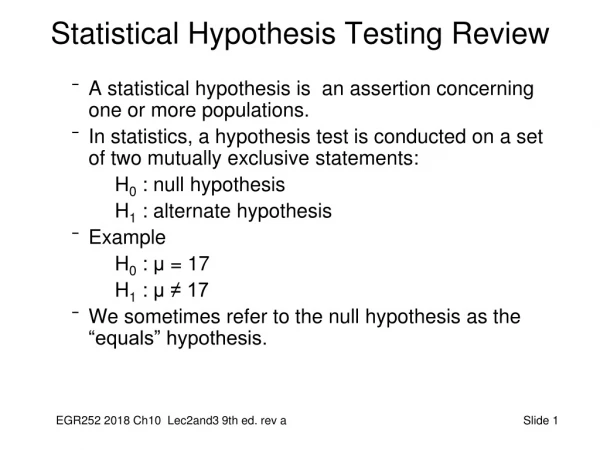
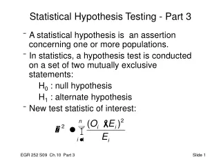
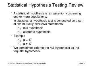
Statistical Hypothesis Testing Review • A statistical hypothesis is an assertion concerning one or more populations. • In statistics, a hypothesis test is conducted on a set of two mutually exclusive statements: H0 : null hypothesis H1 : alternate hypothesis • Example H0 : μ = 17 H1 : μ ≠ 17 • We sometimes refer to the null hypothesis as the “equals” hypothesis.
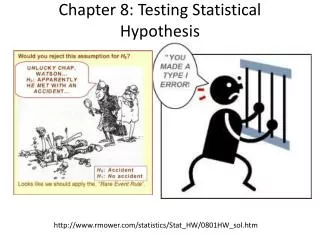
α Probability of committing a Type I error Probability of rejecting the null hypothesis given that the null hypothesis is true P (reject H0 | H0 is true) β Probability of committing a Type II error Power of the test = 1 - β (probability of rejecting the null hypothesis given that the alternate is true.) Power = P (reject H0 | H1 is true) Potential errors in decision-making
Hypothesis Testing – Approach 1 • Approach 1 - Fixed probability of Type 1 error. • State the null and alternative hypotheses. • Choose a fixed significance level α. • Specify the appropriate test statistic and establish the critical region based on α. Draw a graphic representation. • Calculate the value of the test statistic based on the sample data. • Make a decision to reject H0 or fail to reject H0, based on the location of the test statistic. • Make an engineering or scientific conclusion.
Approach 2 - Significance testing based on the calculated P-value State the null and alternative hypotheses. Choose an appropriate test statistic. Calculate value of test statistic and determine P-value. Draw a graphic representation. Make a decision to reject H0 or fail to reject H0, based on the P-value. Make an engineering or scientific conclusion. Hypothesis Testing – Approach 2 p = 0.05 ↓ P-value 0 1.00 P-value 0.75 0.25 0.50
Example: Single Sample Test of the Mean P-value Approach A sample of 20 cars driven under varying highway conditions achieved fuel efficiencies as follows: Sample mean x = 34.271 mpg Sample std dev s = 2.915 mpg Test the hypothesis that the population mean equals 35.0 mpg vs. μ< 35. Step 1: State the hypotheses. H0: μ = 35 H1: μ < 35 Step 2: Determine the appropriate test statistic. σ unknown, n = 20 Therefore, use t distribution
Single Sample Example (cont.) Approach 2: = -1.11842 Find probability from chart or use Excel’s tdist function. P(x ≤ -1.118) = TDIST (1.118, 19, 1) = 0.139665 p = 0.14 0______________1 Decision: Fail to reject null hypothesis Conclusion: The mean is not significantly less than 35 mpg.
Example (concl.) Approach 1: Predetermined significance level (alpha) Step 1: Use same hypotheses. Step 2: Let’s set alpha at 0.05. Step 3: Determine the critical value of t that separates the “reject H0 region” from the “do not reject H0 region”. t, n-1 = t0.05,19 = 1.729 Since H1 specifies “< ” we declare tcrit = -1.729 Step 4: Using the equation, we calculate tcalc = -1.11842 Step 5: Decision Fail to reject H0 Step 6: Conclusion: The mean is not significantly less than 35 mpg.
Your turn … same data, different hypotheses A sample of 20 cars driven under varying highway conditions achieved fuel efficiencies as follows: Sample mean = 34.271 mpg Sample std dev (s) = 2.915 mpg Test the hypothesis that the population mean equals 35.0 mpg vs. μ≠ 35 at an α level of 0.05. Be sure to draw the picture. Step 1 Step 2 Step 3 Step 4 Step 5 Step 6 (Conclusion will be different.)
Two-Sample Hypothesis Testing A professor has designed an experiment to test the effect of reading the textbook before attempting to complete a homework assignment. Four students who read the textbook before attempting the homework recorded the following times (in hours) to complete the assignment: 3.1, 2.8, 0.5, 1.9 hours Five students who did not read the textbook before attempting the homework recorded the following times to complete the assignment: 0.9, 1.4, 2.1, 5.3, 4.6 hours
Two-Sample Hypothesis Testing • Define the difference in the two means as: μ1 - μ2 = d0 where d0 is the actual value of the hypothesized difference • What are the Hypotheses? H0: _______________ H1: _______________ or H1: _______________ or H1: _______________
Our Example Using Excel Reading: n1 = 4 mean x1 = 2.075 s12 = 1.363 No reading: n2 = 5 mean x2 = 2.860 s22 = 3.883 If we have reason to believe the population variances are “equal”, we can conduct a t- test assuming equal variances in Minitab or Excel.
Your turn … • Lower-tail test (μ1 - μ2 < 0) • “Fixed α” approach (“Approach 1”) at α = 0.05 level. • “p-value” approach (“Approach 2”) • Upper-tail test (μ2 – μ1 > 0) • “Fixed α” approach at α = 0.05 level. • “p-value” approach • Two-tailed test (μ1 - μ2 ≠ 0) • “Fixed α” approach at α = 0.05 level. • “p-value” approach Recall
Our Example – Hand Calculation Reading: n1 = 4 mean x1 = 2.075 s12 = 1.363 No reading: n2 = 5 mean x2 = 2.860 s22 = 3.883 To conduct the test by hand, we must calculate sp2 . = 2.803 sp = 1.674 and = ????
Lower-tail test (μ1 - μ2 < 0) Why? • Draw the picture: • Approach 1: df = 7, t0.05,7 = 1.895 tcrit = -1.895 • Calculation: • tcalc = ((2.075-2.860)-0)/(1.674*sqrt(1/4 + 1/5)) = -0.70 • Graphic: • Decision: • Conclusion:
Upper-tail test (μ2 – μ1 > 0)Conclusions • The data do not support the hypothesis that the mean time to complete homework is less for students who read the textbook. or • There is no statistically significant difference in the time required to complete the homework for the people who read the text ahead of time vs those who did not. or • The data do not support the hypothesis that the mean completion time is less for readers than for non-readers.
Our Example Using Excel Reading: n1 = 4 mean x1 = 2.075 s12 = 1.363 No reading: n2 = 5 mean x2 = 2.860 s22 = 3.883 What if we do not have reason to believe the population variances are “equal”? We can conduct a t- test assuming unequal variances in Minitab or Excel.
Another Example: Low Carb Meals Suppose we want to test the difference in carbohydrate content between two “low-carb” meals. Random samples of the two meals are tested in the lab and the carbohydrate content per serving (in grams) is recorded, with the following results: n1 = 15 x1 = 27.2 s12 = 11 n2 = 10 x2 = 23.9 s22 = 23 tcalc = ______________________ ν = ______________ (using equation in table 10.3)
Example (cont.) • What are our options for hypotheses? H0: μ1 - μ2 = 0 or H0: μ1 - μ2 = 0 H1: μ1 - μ2 > 0 H1: μ1 - μ2 ≠ 0 • At an α level of 0.05, • One-tailed test, t0.05, 15 = 1.753 • Two-tailed test, t0.025, 15 = 2.131 • How are our conclusions affected? • Our data don’t support a conclusion that the mean carb content of the two meals are different at an alpha level of .05 (What is H1 ?) • Our data do support a conclusion that Meal 1 has more average carbs than Meal 2 at an alpha level of .05. (What is H1 ?)
Special Case: Paired Sample T-Test Which designs are paired-sample? • Car Radial Belted 1 ** ** Radial, Belted tires 2 ** ** placed on each car. 3 ** ** 4 ** ** • Person Pre Post 1 ** ** Pre- and post-test 2 ** ** administered to each 3 ** ** person. 4 ** ** • Student Test1 Test2 1 ** ** 4 scores from test 1, 2 ** ** 4 scores from test 2. 3 ** ** 4 ** **
Sheer Strength Example* An article in the Journal of Strain Analysis compares several methods for predicting the shear strength of steel plate girders. Data for two of these methods, when applied to nine specific girders, are shown in the table on the next slide. We would like to determine if there is any difference, on average, between the two methods. Procedure: We will conduct a paired-sample t-test at the 0.05 significance level to determine if there is a difference between the two methods. * adapted from Montgomery & Runger, Applied Statistics and Probability for Engineers.
Sheer Strength Example Calculations Hypotheses: H0: μD = 0 H1: μD ≠ 0 t0.025,8 = 2.306 Why 8? Calculation of difference scores (d), mean and standard deviation, and tcalc … d = 0.2739 sd = 0.1351 tcalc = ( d – d0 ) = (0.2739 - 0) = 6.082 sd / sqrt(n) (1.1351 / 3)
What does this mean? • Draw the graphic: • Decision: • Conclusion:
Goodness-of-Fit Tests • Procedures for confirming or refuting hypotheses about the distributions of random variables. • Hypotheses: H0: The population follows a particular distribution. H1: The population does not follow the distribution. Examples: H0: The data come from a normal distribution. H1: The data do not come from a normal distribution.
Goodness of Fit Tests: Basic Method • Test statistic is χ2 • Draw the picture • Determine the critical value χ2 with parameters α, ν = k – 1 • Calculate χ2 from the sample • Compare χ2calcto χ2crit • Make a decision about H0 • State your conclusion
Tests of Independence • Example: 500 employees were surveyed with respect to pension plan preferences. • Hypotheses H0: Worker Type and Pension Plan are independent. H1: Worker Type and Pension Plan are not independent. • Develop a Contingency Table showing the observed values for the 500 people surveyed.
Calculation of Expected Values 2. Calculate expected probabilities P(#1 ∩ S) = P(#1)*P(S) = (200/500)*(340/500)=0.272 E(#1 ∩ S) = 0.272 * 500 = 136
Calculate the Sample-based Statistic Calculation of the sample-based statistic = (160-136)^2/(136) + (140-136)^2/(136) + … (60-32)^2/(32) = 49.63
The Chi-Squared Test of Independence 5. Compare to the critical statistic, χ2α, v where v = (r – 1)(c – 1) Note: v is the symbol for degrees of freedom For our example, suppose α = 0.01 χ2 0.01,2 = ___________ χ2 calc = ___________ Decision: Conclusion:
The Chi-Squared Test in Minitab 15 Chi-Square Test: pp1, pp2, pp3 Expected counts are printed below observed counts Chi-Square contributions are printed below expected counts pp1 pp2 pp3 Total 1 160 140 40 340 136.00 136.00 68.00 4.235 0.118 11.529 2 40 60 60 160 64.00 64.00 32.00 9.000 0.250 24.500 Total 200 200 100 500 • Test statistic: Chi-Sq calc = 49.632, DF = 2, P-Value = 0.000 Reject Ho. • Conclude that worker and plan are not independent.