Download
1 / 23
260 likes | 517 Vues
Evaluating Skill in Ocean Model Parameterizations: Taylor Diagrams. Lynn (Nick) Shay and G. Halliwell MPO, RSMAS, Univ. of Miami PhOD, AOML, NOAA http://isotherm.rsmas.miami.edu/~nick HFIP Observations and Modeling Teams. T’is the Season…….

E N D
Evaluating Skill in Ocean Model Parameterizations: Taylor Diagrams Lynn (Nick) Shay and G. Halliwell MPO, RSMAS, Univ. of Miami PhOD, AOML, NOAA http://isotherm.rsmas.miami.edu/~nick HFIP Observations and Modeling Teams
Ivan’s Track and Intensity Relative to OHC (left) NRL SEED Mooring Locations in Northern Gulf of Mexico Relative to Bottom Depth (Right) (Teague et al., JPO, 2007). 14 ADCP moorings- Focus here in Array 9.
Ocean Structure Gulf Versus East Pacific Strong vertical temperature, salinity and density gradients at base of OML in EPAC… Implications for mixing…and ocean (SST) cooling. N~20 cph
Differentiated cooling in the LC system (Jaimes and Shay, MWR, 2009) T ~ -1oC T ~ -4.5oC Loop Current Shedding front T ~ -0.5oC Warm core eddy Cluster-averaged temperature profiles vertical shear (s-2) ageostrophic velocity (cm s-1) ageostrophic KE (cm2 s-2) Richardson number
Taylor Diagrams: Taylor diagram R E Taylor, K., 2001: JGR, 106, D7, 7183-7192
Taylor Diagram – Skill Score Taylor diagram S-isolines: 0.1 intervals, grey shading Taylor, K., 2001: JGR, 106, D7, 7183-7192
MOTIVATION: Ivan (2004) over the GOM SSH (cm) from HYCOM (from Halliwell et al., MWR, 2008). SST Analyses Northern Cyclone Southern Cyclone
HYbrid Coordinate Ocean Model (HYCOM)Hurricane Ivan Simulations 10 Sept-6 Oct 04 • Configuration: • 0.04° Mercator grid, Gulf of Mexico domain • No data assimilation performed • Initial and boundary conditions from U.S. Navy HYCOM ocean nowcast-forecast system: • Data assimilative ocean nowcast • Navy Coupled Ocean Data Assimilation (NCODA) assimilation • Atmospheric Forcing: • Navy 27 km COAMPS atmospheric model • Vector wind blended with higher resolution fields from HWIND • Wind stress for HWIND calculated using Donelan cd
TMI and KPP SST Comparisons Pre Ivan SST Post-Ivan SST Pre-Post Ivan ΔSST
Observed/Simulated Current Response at M9 (1.5 Rmax) from 7 Experiments Halliwell et al., MWR, (2009) Below cd using ocean response as a tracer in Shay and Jacob (2006)
Current Time Series Comparisons @ 1.5 Rmax U (east-west) V (north-south)
Taylor Diag., simulations vs. baseline: SST; v Current at M9 (1.5Rmax). (Halliwell et al., MWR, 2009)
Taylor Diag., simulations vs. observations: SST; v Current at M9 (1.5Rmax). (Halliwell et al., MWR, 2009)
Track and Intensity of TC’s Gustav and Ike Versus AXBTs relative to OHC and 26oC Isotherm Depth. Gustav : 191 AXBTs 111 GPS Drifters Floats Ike : 216 AXBTs 111 GPS Drifters Floats (Shay et al. 2009)
NOAA WP-3D Profiling over MMS Moorings (Collaboration with AOML HRD, AOC, TPC, NCEP) Deliverables include: V, T, S profiles to 1000 m @ 2-m resolution. Surface winds (SFMR, GPS) provided by HRD. Atmospheric profiles of V, T and RH @ 5-m resolution. • Goal: To observe and improve our understanding of the LC response to the near-surface wind structure during TC passages. Specific objectives are: • Determine the oceanic response of the LC to TC forcing; and, • Influence of the LC response on the atmospheric boundary layer and intensity.
Progress and Blueprint For Future Ivan a clear example of negative feedback(wake cooling/mixing induced by strong winds and Cold Core Ring) as opposed to positive feedback over the Loop Current and Warm Core Rings. Taylor Diagrams collapse Standard Deviation, Correlation Indices and RMS Differences into one representation relative to an observation of current, temperatures, winds, humidities, variance etc to assess model performance. Estimate skill by combining standard deviations and correlations. In Ivan case, 14 sets of model simulations were made differing in only one aspect at a time. Approach shows sensitivity and allows us to isolate physics (Even a 1-D versus 3-D Ocean!) Applying same approach to OHC variability in assessing uncertainties in satellite retrievals using in situ data as truth. Field programs to acquire 3-D data……