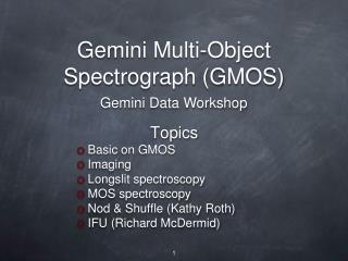
Gemini Multi-Object Spectrograph (GMOS)
Gemini Multi-Object Spectrograph (GMOS). Gemini Data Workshop. Topics Basic on GMOS Imaging Longslit spectroscopy MOS spectroscopy Nod & Shuffle (Kathy Roth) IFU (Richard McDermid). 1. GMOS Overview. GMOS detectors: three 2048x4608 E2V chips (6144 x 4608 pixels)

Gemini Multi-Object Spectrograph (GMOS)
E N D
Presentation Transcript
Gemini Multi-Object Spectrograph (GMOS) Gemini Data Workshop • Topics • Basic on GMOS • Imaging • Longslit spectroscopy • MOS spectroscopy • Nod & Shuffle (Kathy Roth) • IFU (Richard McDermid) 1
GMOS Overview • GMOS detectors: • three 2048x4608 E2V chips (6144 x 4608 pixels) • 0.0727” (GMOS-N) and 0.073” (GMOS-S) per pix • Gaps between CCDs - 37 unbinned pixels. • Field of view: 5.5’ x 5.5’ (imaging) • Filters • Sloan u’ (GMOS-S only) g’ r’ i’ z’ and CaIII • Hα, HαC, HeII, HeIIC, OIII, OIIIC, SII (Narr. band) • Others: GG445, OG515, RG610, RG780, DS920 • Spectroscopy • Longslits (0.5” - 5.0”), MOS and IFU • Nod & Shuffle 2
GMOS Overview • Available gratings Grating turret supports only 3 gratings + mirror 3
GMOS Overview • GMOS detectors characteristics • Good cosmetic, with only few bad pixels • Bad pixels masks for imaging - provided by the observatory (1x1 and 2x2) - gmos$data/ directory • Saturation level: ~64000 ADU • Linearity - ~60.000 ADU (<1%) • CCD readouts and gains configurations • Slow readout/low gain (science) • Fast readout/low gain (bright obj.) • Fast readout/high gain • Slow readout/high gain (eng. only) • Readout time: • 1x1 slow/low - 129 sec • 2x2 slow/low - 37 sec 4
to the detector Mask assembly with cassettes and masks Grating turret Filter wheels 5
Integral Field Unit Cassette # 1 OIWFS and patrol field area
GMOS Data Reduction General guidelines • Fetch your program using the OT • Check for any note added by the observer(s) and/or the Queue Coordinator(s) regarding your observations • Check the observing log (you can use the OT) • Look at your raw data • Check all frames • use imstatistic, implot or other IRAF tasks to check the data
GMOS Data Reduction Calibrations • Set of Baseline Calibrations provided by the observatory • Bias for all modes of observations • Twilight flats: imaging and spectroscopy • Spectroscopic flats from GCAL unit • CuAr Arcs for spectroscopy (GCAL unit) • Nighttime calibrations (baseline) • Photometric standard stars - zero point calibrations • Flux standard - flux calibration • Other calibrations (charged to the program) • Radial velocity standards • Lick standards, etc.
GMOS Images: example HCG 87: g’, r’ and i’ filters, 1 x 1 (no binning) Calibrations Reduction Steps • Combine bias (trim, overscan) • Twilight flats : subtract bias, trim, overscan, combine • Reduce images: bias, overscan, trimmed, flatfield • Fringing correction: i’-band only • Mosaic the images and combine the frames by filter
Reducing GMOS Images Bias reductions (for all modes) • Be sure to use the correct bias • slowreadout/low gain • binning: 1x1 • Tip: check keyword AMPINTEGin the PHU • AMPINTEG = 5000 – Slow • AMPINTEG = 1000 – fast • Gain -- in the header • CCDSUM - binning • Bias reductions -- uses gbias • Overscan subtr. – recommended • gbias @bias.list bias_out.fits fl_trim+ fl_over+ rawpath=dir$ • Check the final combined bias image
Reducing GMOS Images Twilight flats • Twilight flats are used to flat field the images • twilight flats are observed periodically for all filters • Special dithering pattern • Constructing flat field with giflat • giflat @flat_g.lst outflat=gflat fl_trim+ fl_over+ rawpath=dir$ • The default parameters work ok for most cases • Final flat is normalized
Reducing GMOS Images Fringing correction • Significant fringing in i’ and z’ filters • Blank fields for fringing removal • observed every semester in i’ and z’ • Best fringing correction - use the same science images • Constructing the fringing frame • With gifringe using bias, overscaned, trimmed and flatfielded images. • gifringe @fring.lst fringeframe.fits • Removing the fringing • girmfringe @inp.lst fringeframe.fits • Output = Input - s * F
Reducing GMOS Images Science images • Reducing the images with gireduce • gireduce: gprerare, bias, overscan and flatfield the images • gireduce @obj.lst fl_bias+ fl_trim+ fl_flat+ fl_over+ bias=bias.fits flat1=flatg flat2=flatr flat3=flati rawpath=dir$ • Removing fringing with girmfringe (i’ band images only) • Inspect all images with “gdisplay” • Mosaicing the images with gmosaic - > gmosaic @redima.lst • Combining your images using imcoadd • imcoadd - search for objects in the images, derive a geometrical trasformation (shift, rotation, scaling), register the objects in the images to a common pixel position, apply the BPM, clean the cosmic ray events and combine the images
Final GMOS image HCG 87
GMOS MOS Spectroscopy GCAL flats + CuAr arc – inserted in the sequence
GMOS Mask Definition File (MDF) • Contains information about • Slit locations, slit width, slit length, tilt angle, etc • RA, Dec position of the objects • X, Y position of the objects in the pre-imaging • Necessary for data reduction
GMOS MOS Gcal flat Wavelength coverage: ~ 456nm – 884nm CCD2 CCD1 CCD3 Red Blue Significant fringing above 700nm
GMOS MOS Spectra Alignment stars
GMOS MOS reduction • Basic reduction steps • Prepare the images by adding the MDF file with gprepare • Bias subtraction for all images, including the CuAr arcs • Cuar arcs observed during the day - then an overscan subtraction is enough. • Bias subtraction is performed with gsreduce • gsreduce@obj.lst fl_flat- fl_gmosaic- fl_fixpix- \ fl_gsappw- fl_cut- fl_over+ fl_bias+ bias=biasima.fits \ rawpath=dir$ mdfdir=dir$
GMOS MOS reduction • Wavelength Calibration • Wavelength calibration is performed slit by slit • Do the calibration interactively - recommended • Mosaic the CuAr arc with gmosaic • cut the spectra with gscut • gscut mCuArarc outimage=cmCuAr secfile=cmCuAr.sec • Inspect the cmCuAr.sec file and the image to see if the cut is good • If the cut is not good, then adjust the yoffset param.
GMOS MOS reduction • Wavelength Calibration • Establish wavelength calibration with gswavelength • gswavelegth • Call gsappwave to perform an approximate wavelength calibration using header information • Use autoidentify to search for lines • CuAr_GMOS.dat – line list • Run reidentify to establish the wavelength calibration • Call fitcoords to determine the final solution (map the distortion). • Important parameters – step (see Emma’s talk). • For MOS – recommended “step=2” – reidentification of the lines is performed every two lines • Use a low order for the fit
GMOS MOS reduction • Flat field • Use gsflat to derive the flat field for the spectra • gsflat - generate a normalized GCAL spectroscopic flatfield. • gsflat - remove the GCAL+GMOS spectral response and the GCAL uneven illumination from the flat-field image and leave only the pixel-to-pixel variations and the fringing. • gsflat inpflat outflat.fits fl_trim- fl_bias- fl_fixpix- \ fl_detec+ fl_inter+ order=19 • Function spline3 and order=19 work ok (you don’t want to remove the fringing from the flat) • Test with other orders and functions.
GMOS MOS reduction Normalized Flat field
GMOS MOS reduction • Bad Pixel Mask • There is not BPM for spectroscopy • gbpm works only for direct imaging • You can minimize the effect of the bad pixels in your spectra by generating your own BPM • The BPM will contain only bad pixels, not hot pixels. • An example is given in the GMOS MOS Tutorial MOS data • The BPM is constructed separately for each CCD.
GMOS MOS reduction • Reducing the spectra • Calling gsreduce and gscut to flatfield and cut the slits • gsreduce specimage fl_trim- fl_bias- fl_gmosaic+ fl_fixpix+ fl_cut+ fl_gsappwave- flat=flatnorm.fits • Cleaning cosmic rays using the Laplacian Cosmic Ray Identification routine by P. van Dokkum • see http://www.astro.yale.edu/dokkum/lacosmic/ • Calibrating in wavelength and rectifying the spectra using gstransform • gstransform crcleanspecimage wavtraname=”refarc" fl_vardq-
GMOS MOS reduction Reduced spectra After cosmic ray removal gstransform-ed Tilted slit
GMOS MOS reduction • Extracting the spectra • Sky subtraction • can use gsskysub on 2-D transformed image • can use gsextract to perform the sky subtraction • Using gsextract • gsextract txspec.fits fl_inter+ background=fit torder=5 tnsum=150 tstep=50 find+ apwidth=1.3 recenter+ trace+ fl_vardq- weights="variance" border=2 • Critical parameters: apwidth, background region and order of the background fit (1 or 2) • Background region can be selected interactively • In this example the aperture width is 1.3”
Find the spectrum background region Extracted spectrum Sky lines
GMOS MOS reduction • What is next … • Check all spectra • Check wavelength calibrations using the sky lines • Combining the spectra – scombine recommended • Analyze the results
GMOS Longslit reduction • Longslit reduction is a particular case of MOS reduction for ONE slit • The reduction is performed exactly in the same way as for MOS spectroscopy. • gprepare the images by adding the MDF file • Bias subtraction for all images • Establish wavelength calibration and flat normalization • gsreduce to reduce the spectrum • Cosmic ray removal • Calibrating in wavelength and rectifying the spectra using gstransform • Extracting the spectrum • Tutorial data for Flux standard • Additional steps – derive sensitivity function (gsstandard)