Download
1 / 48
480 likes | 662 Vues
PCFG Induction. James Scicluna Colin de la Higuera University of Nantes. Outline. About grammatical inference and distributions Why learn ? Some motivations About probabilistic context -free grammars What is a PCFG? Parsing issues Distances Strongly contextual PCFGs

E N D
PCFG Induction James Scicluna Colin de la Higuera University of Nantes
Outline • About grammatical inference and distributions • Whylearn? • Some motivations • About probabilisticcontext-free grammars • Whatis a PCFG? • Parsing issues • Distances • StronglycontextualPCFGs • Inside-Outside • Algorithm COMINO • General idea • An over-generalgrammar • Reducing the size • Computing the weights • Experiments • Artificial data • WSJ • Furtherremarks • Can a PCFG model naturallanguage?
Grammatical inference Applications The « need » of probabilities 1. About grammatical inference and distributions
Grammatical inference Goal is to learn sets of (rewrite) rules given structured data (strings, trees, graphs) Typical task is to learn finite state machines More complex task is to learn context-free grammars: of special use for natural language processing
A linguistic tree. (Courtesy of Mark Knauf and Etsuyo Yuasa, Department of East Asian Languages and Literatures (DEALL), Ohio State University.)
An NLP task • Given raw text build a model such that for a given sentence • Prediction is good: this is used for disambiguation (the probability of a correct sentence is higher that the probability of an incorrect sentence): have low perplexity • The parse tree is right (the number of correct sub-trees is large)
Ambitious goal • Suppose the grammar is context-free and probabilistic • This is a PCFG • Hard • There exists an algorithm (inside-outside) allowing to estimate the weights given some data and a CFG • But where does the CFG come from?
2.1 Definitions 2.2 Equivalence between models 2.3 Parsing issues 2.4 Distances 2.5 NTS 2. About probabilistic context-free grammars
2.1 Distributions, definitions Let D be a distribution over * 0PrD(w)1 w*PrD(w)=1
A Probabilistic Context-Free Grammar is a <N, , I, R, P > • N set of nonterminal symbols • IN the initial symbols • R is a finite set of rules N(N)* • P: I[0;1]
Notations • Derives in one step • f (S,)R • is the reflexive and transitive closure of • whereu*,N • Pr()=where (Si,) is the rulebeignused • Probability of a string is the sum of the probabilities of all the left-mostderivations of • L(S)= • L(G)=
What does a PCFG do? (by the way, this grammar is inconsistent as Pr(*=0.25) S S S S S S It defines the probability of each string w as the sum (over all possible parse trees having w as border) of the products of the probabilities of the rules being used. S SS (0.8) | a (0.2) Pr(aaa)=0,01024 a S S a S S a a a a
How useful are these PCFGs? They can define a distribution over * They do not tell us if a string belongs to a language They seem to be good candidates for grammar induction
2.3 Parsing issues Computation of the probability of a string or of a set of strings You can adapt CKY or Earley
CKY • Needs a Chomsky (or quadratic normal form) • Transforming a PCFG into an equivalent PCFG in Chomsky normal form can be done in polynomial normal form • Example • S abSTb (0.63) is transformed into • S aS1 (0.63) • S1 bS2 (1) • S2 SS3 (1) • S3 Tb (1)
2.4 Distances: recent results • What for? • Estimate the quality of a language model • Have an indicator of the convergence of learning algorithms • Use it to decide upon non-terminal merging • Construct kernels • Computing distances between PCFGs corresponds to solving undecidable problems
Equivalence TwoprobabilisticgrammarsG1and G2are (language) equivalent if x*, PrG1(x)=PrG2(x). Wedenote by EQ, PCFGclassthe decisionproblem: are twoPCFGs G1and G2equivalent?
Co-emission and treecoemission • The coemissionof two probabilistic grammars G1 and G2is the probability that both grammars G1 and G2simultaneously emit the same string: • COEM(G1,G2)= x*PrG1(x)PrG2(x) • A particular case of interest is the probability of twice generating the same string when using the same grammar: Given a PCFG G, the auto-coemissionof G, denoted as AC(G), is COEM(G,G). • We introduce the tree-auto-coemissionas the probability that the grammar produces exactly the same left-most derivation (which corresponds to a specific tree): • Given a PCFG G, the tree-auto-coemissionof G is the probability that G generates the exact same left-most derivation twice. We denote it by TAC(G). • Note that the tree-auto-coemission and the auto-coemission coincide if and only if G is unambiguous: • Let G be a PCFG. • AC(G)TAC(G). • AC(G)=TAC(G) iff G is unambiguous.
Some distances (1) The L1distance (or Manhattan distance) betweentwoprobabilisticgrammars G1 and G2is: dL1(G1, G2)=x*|PrG1(x)-PrG2(x) | The L2distance (or Euclidian distance) betweentwoprobabilisticgrammars G1 and G2is: dL2(G1, G2)= L2distance canberewritten in terms of coemission, as: dL2(G1, G2)=
Some distances (2) • The Ldistance (or Chebyshevdistance) betweentwoprobabilisticgrammars G1 and G2is: • dL(G1, G2)=maxx* |PrG1(x)-PrG2(x)| • Note that the Ldistance seemscloselylinkedwith the consensus string, whichis the most probable string in a language. • The variation distance betweentwoprobabilisticgrammars G1 and G2is: • dV(G1, G2)=maxX* xX(PrG1(x)-PrG2(x)) • The variation distance looks likedL, but isactuallyconnectedwithdL1: dV(G1, G2)=½dL1(G1, G2) • A number of distances have been studiedelsewhere (for example \cite{jago01,cort07}): • The Hellinger distance (dH) • The Jensen-Shannon (JS) distance (dJS) • The chi-squared (2) distance (d2)
Decisionproblems for distances Wedenote by dX, PCFGclass the decisionproblem: Is d(y,z)…
Kullback-Leibler divergence The Kullback-Leibler divergence, or relative entropyis not a metric: The KL divergence betweentwoprobabilisticgrammarsG1 and G1 is: dKL(G1,G2)=x*PrG1(x)(log PrG1(x) – log PrG2(x)) Evenif the KL-divergence does not respect the triangularinequality, dKL(G1, G2)=0 iffG1 G2. Let G be a PCFG. The consensus string for G is the most probable string of DisG. Wedenote by CS, PCFGclassthe decisionproblem: isw the most probable string givenG?
Theorem dL1, PCFGclass, dV, PCFGclass, dH, PCFGclass,dJS, PCFGclass are undecidable Sketch of proof If not, thenwecouldeasilysolve the emptyintersection problem of 2 CFGsby building Mp(G) and Mp(G') and thenchecking if dL1(Mp(G),Mp(G'))=2.
2.5 Strongly congruential grammars • The hypothesis is that substrings are substitutable • The dog eats • The cat eats dog and cat are substitutable and will derive from the same non terminal
A bit more mathematical If Pr( xdogy | dog )=Pr( xcaty | cat ) (x y) then dog cat If for each S in N, L(S) is exactly one class, the grammar is strongly contextual. The notation |cat is dodgy: cat can appear various times in a sentence and should be counted each time.
General algorithm Initializeweights Prev_ll LL(G,T) Whiletrue do E-step M-step LikelihoodLL(G,T) If likelihood-prev-likelihood<then return G Prev_lllikelihood
Loglikelihood LL(G,T)=xTlogPrG(x)
E-step • For eachA in R do • Count(A) 0 • For eachw in T do • Count(A ) Count(A )+Ew[A] • WhereEw[A] is the insideprobability • Goal of the E-stepis to parse the sample
M-step • For each A in R do • P(A) • Goal of the M stepisjust to use the counts to define the new weights
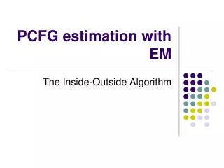
Computing the insideprobability This is Pr(A=>*v) If Gis in CNF, thisisexactlywhat CYK does
Computing the outsideprobability This is Pr(A=>*uBw)
3.1 Building an over general grammar 3.2 Minimizing 3.3 Estimating probabilities 3 COMINO
3 steps Step 1 Use the data to build a congruence over all the substrings using statistical contextual evidence This leads to a first over-general grammar Step 2 Use constraint programming to minimize this grammar, ie select a minimum number of rules/non-terminals such that the grammar generates the data Step 3 Estimate the probabilities using inside-outside
Step 1 Buildfrom a sample all possible rules in CNF (abc leads to SabcSaSbc and SabcSabSc ) Mergenonterminals if they are equivalent Equivalent: same distributions Note: for a number of reasonswe use k-contexts: ksymbols to eachside
Sample {ab, aabb, aaabbb} Congruence Classes • 1: [a], • 2: [b], • 3: [ab, aabb, aaabbb], • 4: [aa], • 5: [bb], • 6: [aab, aaabb], • 7: [abb, aabbb], • 8: [aaa], • 9: [bbb], • 10: [aaab], • 11: [abbb]
Step 2 Boolean Formula One variable (conditional statement) per substring. For example, X6(X1X3)(X4X2) represents the two possible ways aabin congruence class 6 can be split (a|ab, aa|b). The statement X3 (X1X7)(X4X5)(X6X2) represents the three possible ways aabbin congruence class 3 can be split (a|abb, aa|bb, aab|b).
Sample {ab, aabb, aaabbb} Congruence Classes BooleanFormula Variables X1, X2and X3are true. X3(X1X2) X3(X1X7)(X4X5) (X6X2) X3(X1X7)(X4X11)(X8X9)(X10X5)(X6X2) X4(X1X1) X5(X2X2) X6(X1X3) (X4X2) X6(X1X3)(X4X7)(X8X5)(X10X2) X7(X1X5) (X3X2) X7(X1X11)(X4X9)(X6X5) (X3X2) X8(X1X4) (X4X1) X9(X2X5) (X5X2) X10(X1X6) (X4 X3) (X8X2) X11(X1X9) (X3X5) (X7X2) • 1: [a], • 2: [b], • 3: [ab, aabb, aaabbb], • 4: [aa], • 5: [bb], • 6: [aab, aaabb], • 7: [abb, aabbb], • 8: [aaa], • 9: [bbb], • 10: [aaab], • 11: [abbb]
Running the solver on this formula will return the following true variables that make up a minimal solution: X1, X2, X3and X7. • Grammar • X3is the starting non-terminal • X3 X1 X7 | X1 X2 • X7 X3 X2 • X1a • X2 b • (equivalent to X3 a X3 b| ab )
Someformallanguages for the experiments UC1 : { anbn: n0} UC2 : { anbncmdm: n, m0} UC3 : { anbm : nm } UC4 : { apbq: pq } UC5 : Palindromes over alphabet {a,b}with a central marker UC6 : Palindromes over alphabet {a,b} without a central marker UC7 : Lukasiewicz language(Sa S S| b)
Ambiguousgrammars AC1 : {w: |w|a= |w|b} AC2: {w: 2|w|a= |w|b} AC3: Dyck language AC4: Regular expressions
Artificial NLP grammars NL1 : Grammar ’a’, Table 2 in [LS00] NL2 : Grammar ’b’, Table 2 in [LS00] NL3 : Lexical categories and constituency, pg 96 in [Sto94] NL4 : Recursiveembeddingof constituents, pg 97 in [Sto94] NL5 : Agreement, pg98 in [Sto94] NL6 : Singular/plural NPs and numberagreement, pg 99 in [Sto94] NL7 : Experiment 3.1 grammarin [ATV00] NL8 : Grammar in Table 10 [ATV00] NL9 : TA1 grammarin [SHRE05].
Some goals achieved A betterunderstanding of what PCFG learningwas about Experimentalresultsshowing an increase in performance with respect to established state of the art methods Another use of solvers in grammatical inference
Some lessons learnt Merge, then reduce the search space Is a PCFG a good model for NL? A bad research topic is one which is difficult but looks easy