Download
1 / 30
330 likes | 489 Vues
One-way Analysis of Variance. 1-Factor ANOVA. Previously…. We learned how to determine the probability that one sample belongs to a certain population. Then we learned how to determine the probability that two samples belong to the same population. Now….

E N D
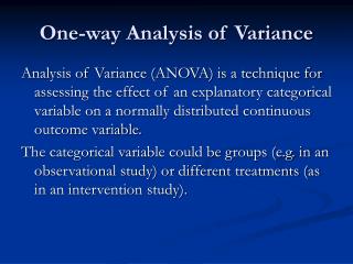
One-way Analysis of Variance 1-Factor ANOVA
Previously… • We learned how to determine the probability that one sample belongs to a certain population. • Then we learned how to determine the probability that two samples belong to the same population.
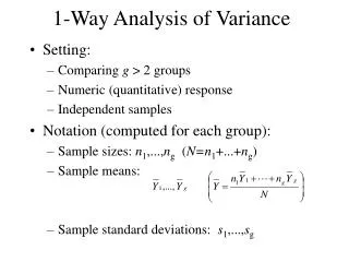
Now… • We will learn how to determine the probability that two or more samples were taken from the same population. • While the t tests use standard deviation units (standard error of the mean and standard error of the difference), this new analysis uses variance.
One-Way Analysis of Variance • One-way (or one factor) just means that we are looking at the effect of one independent variable. • With an ANOVA, we can partition the variance into categories to determine how much of the variance is due to our experimental procedure and how much is due to individual differences or experimental error. • Instead of a t score, the ANOVA produces an F score, which has its own table.
One-way ANOVA Hypothesis • The null hypothesis for the ANOVA with three groups is: • H0: μ1 = μ2 = μ3 • The alternative hypothesis is: • H1: μ1 ≠ μ2 ≠ μ3
One-way ANOVA Hypothesis • Notice, at the end of the ANOVA, we cannot say which group’s results are responsible for rejecting the null. • To do that, we have to conduct a post hoc analysis, which we will get to later.
Terms refers to a raw score from a group (g). refers to the mean of a group. refers to the mean of all scores in all groups or the “grand mean.”
Key Deviations • Remember we use deviation scores to find sum of squares (SS) and SS to find variance. The mean score for a group minus the grand mean. A raw score in a group minus the group mean. A raw score minus the grand mean.
Picturing the Variability • If you have only a little within-groups variability, but a lot of between groups variability, it is easy to see that there is an effect. • If you have a lot of within groups variability, but only a little between groups variability, it is hard to see that there is an effect. • See p. 241.
Picturing the Variability Between Groups Variability Within Groups Variability Total Variability
Three Sources of Variability • Individual Differences • Experimental Error • Treatment Effect Within Groups Variability Between Groups Variability
Sum of Squares • To run the ANOVA, we are going to first find the sum of squares for each variance of interest. Total SS: Within-groups SS: Between-groups SS:
Between-groups SS • This one might need a little explaining: • All it means is that you subtract the grand mean from the group mean and square the result, then multiply it times the group N. Do this for each group and add them up.
Step 1: Find SS Group 1 Mean = 5 Group 2 Mean = 9 Grand Mean = 7
Step 2: ANOVA Summary Table K = # of groups
Step 3: Find Fcrit • Look at Table C in Appendix 4 • Find the column associated with dfb • Find the row associated with dfw • In our example, the critical value at the .05 level is 5.99, and 13.7 at the .01 level.
Step 4: Make a Decision • If we set α = .05, we can reject the null because Fobt (7.38) is bigger than Fcrit(5.99). • If we set α = .01, we retain the null because Fobt (7.38) is smaller than Fcrit(13.7).
Step 5: Interpret the Results • Because the obtained F is larger than the critical value at the .05 level, we reject the hypothesis that the samples came from the same population and conclude that the treatments varied in their effectiveness. • Because the obtained F is smaller than the critical value at the .01 level, we retain the hypothesis that the samples came from the same population and conclude that the treatments did not vary in their effectiveness.
What is F? • F is the ratio of variability between groups to variability within groups. (MSb/MSw) • If the samples came from the same population, we would expect both between and within group variability to be about the same, so we would expect F to be 1. • If the samples do not come from the same population, we would expect the between group variability to be greater than the within group variability, which would make F bigger (because between group variability is in the numerator).
What is F? • Also, just in case you were wondering, if you ran an independent samples t test on the data in our example (remember we had only two groups), you would get the same exact results. • This is because the math behind the 1-way ANOVA and the 2-sample t test is the same.
Activity #1 Number of tasks completed: • Group 1 (downers) = 4, 1, 5, 2 • Group 2 (placebo) = 5, 6, 8, 9 • Group 3 (uppers) = 8, 7, 9, 8
Now What? • We rejected the null, so we are pretty sure that μ1 ≠ μ2 ≠ μ3.In other words, we are pretty sure that people in one of the groups are somehow different from people in another group, but we don’t know which groups. • We need to do a post hoc analysis. There are many of them, but we will talk about the Fisher LSD.
Fisher LSD (Least Significant Difference) Test • The reason we don’t just run a bunch of t tests when we have more than two groups to compare is that we increase the probability of Type I Error (incorrectly rejecting the null). • Why is this? • Because, the probability of finding a difference between groups 1 and 2 OR groups 1 and 3 OR groups 2 and 3 is much greater than the probability of finding a difference between any two of the groups (remember the addition rule of probability).
Fisher LSD (Least Significant Difference) Test • The Fisher LSD increases the difference required to find a significant result. • Here is the formula: • Get tfrom the table using df= N – K. • N1 and N2 are the sample sizes for the first and second samples we are comparing.
Fisher LSD (Least Significant Difference) Test • For three groups, you will have three comparisons: • Group 1 mean – Group 2 mean • Group 1 mean – Group 3 mean • Group 2 mean – Group 3 mean
Fisher LSD (Least Significant Difference) Test • If all of your sample sizes are the same, you will only need to compute LSD once. • Remember what LSD means, and it will make sense. Least significant difference means the smallest difference between the sample means that can be significant.
Fisher LSD (Least Significant Difference) Test • If the difference between the group means you are comparing is at least as large as your obtained LSD, then the difference between those groups is “significant” at the alpha level you used.
Activity #2 • Using α = .01, conduct a LSD post hoc analysis on our activity #1 data. • Interpret the results.
Homework • Study for Chapter 11 Quiz • Read Chapter 12 • Do Chapter 11 HW