Understanding Routing and Forwarding in Network Algorithms
This overview explains the critical distinction between routing and forwarding in networking. Forwarding is the process of sending packets along the physical path, while routing determines the optimal pathways for traffic. The presentation includes principles of routing algorithms, focusing on decentralized systems and properties that enhance efficiency, such as addressing pitfalls in packet transmission. Dijkstra's algorithm is highlighted as a key method for finding the shortest paths in networks by evaluating link costs and optimizing routes for better performance.


Understanding Routing and Forwarding in Network Algorithms
E N D
Presentation Transcript
Routing versus Forwarding • Forwarding is the process of sending a packet on its way • Routing is the process of deciding in which direction to send traffic Forward! Which way? Which way? packet Which way? CSE 461 University of Washington
Improving on the Spanning Tree • Spanning tree provides basic connectivity • e.g., some path BC • Routing uses all links to find “best” paths • e.g., use BC, BE, and CE Unused B B A A C C D D E E F F CSE 461 University of Washington
Goals of Routing Algorithms • We want several properties of any routing scheme: CSE 461 University of Washington
Rules of Routing Algorithms • Decentralized, distributed setting • All nodes are alike; no controller • Nodes only know what they learn by exchanging messages with neighbors • Nodes operate concurrently • May be node/link/message failures Who’s there? CSE 461 University of Washington
Delivery Models • Different routing used for different delivery models Unicast (§5.2) Multicast (§5.2.8) Broadcast (§5.2.7) Anycast (§5.2.9) CSE 461 University of Washington
Shortest Path Routing (§5.2.1-5.2.2)
Topic F • Defining “best” paths with link costs • These are shortest path routes E G D A B H C Best? CSE 461 University of Washington
What are “Best” paths anyhow? F • Many possibilities: • Latency, avoid circuitous paths • Bandwidth, avoid slow links • Money, avoid expensive links • Hops, to reduce switching • But only consider topology • Ignore workload, e.g., hotspots E G D A B H C CSE 461 University of Washington
Shortest Paths We’ll approximate “best” by a cost function that captures the factors • Often call lowest “shortest” • Assign each link a cost (distance) • Define best path between each pair of nodes as the path that has the lowest total cost (or is shortest) • Pick randomly to any break ties CSE 461 University of Washington
Shortest Paths (2) F • Find the shortest path A E • All links are bidirectional, with equal costs in each direction • Can extend model to unequal costs if needed 2 4 E G 3 10 3 2 D 4 1 A B 4 2 2 H C 3 CSE 461 University of Washington
Shortest Paths (3) F • ABCE is a shortest path • dist(ABCE) = 4 + 2 + 1 = 7 • This is less than: • dist(ABE) = 8 • dist(ABFE) = 9 • dist(AE) = 10 • dist(ABCDE) = 10 2 4 E G 3 10 3 2 D 4 1 A B 4 2 2 H C 3 CSE 461 University of Washington
Shortest Paths (4) F • Optimality property: • Subpaths of shortest paths are also shortest paths • ABCE is a shortest path So are ABC, AB, BCE, BC, CE 2 4 E G 3 10 3 2 D 4 1 A B 4 2 2 H C 3 CSE 461 University of Washington
Sink Trees F • Sink tree for a destination is the union of all shortest paths towards the destination • Similarly source tree 2 4 E G 3 10 3 2 D 4 1 A B 4 2 2 H C 3 CSE 461 University of Washington
Sink Trees (2) F • Implications: • Only need to use destination to follow shortest paths • Each node only need to send to the next hop • Forwarding table at a node • Lists next hop for each destination • Routing table may know more 2 4 E G 3 10 3 2 D 4 1 A B 4 2 2 H C 3 CSE 461 University of Washington
Dijkstra’s Algorithm Algorithm: • Mark all nodes tentative, set distances from source to 0 (zero) for source, and ∞ (infinity) for all other nodes • While tentative nodes remain: • Extract N, the one with lowest distance • Add link to N to the shortest path tree • Relax the distances of neighbors of N by lowering any better distance estimates CSE 461 University of Washington
Dijkstra’s Algorithm (2) F • Initialization ∞ 2 4 E G 3 ∞ ∞ 10 3 2 D 4 1 ∞ A B 0 4 ∞ 2 2 H We’ll compute shortest paths to/from A C 3 ∞ ∞ CSE 461 University of Washington
Dijkstra’s Algorithm (3) F • Relax around A ∞ 2 4 E G 3 ∞ 10 10 3 2 D 4 1 ∞ A B 0 4 4 2 2 H C 3 ∞ ∞ CSE 461 University of Washington
Dijkstra’s Algorithm (4) F • Relax around B Distance fell! 7 2 4 E G 3 7 8 10 3 2 D 4 ∞ 1 A B 0 4 4 2 2 H C 3 6 ∞ CSE 461 University of Washington
Dijkstra’s Algorithm (5) F • Relax around C Distance fell again! 7 2 4 E G 3 7 7 10 3 2 D 4 8 1 A B 0 4 4 2 2 H C 3 6 9 CSE 461 University of Washington
Dijkstra’s Algorithm (6) F • Relax around G Didn’t fall … 7 2 4 E G 3 7 7 10 3 2 D 4 8 1 A B 0 4 4 2 2 H C 3 6 9 CSE 461 University of Washington
Dijkstra’s Algorithm (7) F • Relax around F Relax has no effect 7 2 4 E G 3 7 7 10 3 2 D 4 8 1 A B 0 4 4 2 2 H C 3 6 9 CSE 461 University of Washington
Dijkstra’s Algorithm (8) F • Relax around E 7 2 4 E G 3 7 7 10 3 2 D 4 8 1 A B 0 4 4 2 2 H C 3 6 9 CSE 461 University of Washington
Dijkstra’s Algorithm (9) F • Relax around D 7 2 4 E G 3 7 7 10 3 2 D 4 8 1 A B 0 4 4 2 2 H C 3 6 9 CSE 461 University of Washington
Dijkstra’s Algorithm (10) F • Finally, H … 7 2 4 E G 3 7 7 10 3 2 D 4 8 1 A B 0 4 4 2 2 H C 3 6 9 CSE 461 University of Washington
Dijkstra Comments • Dynamic programming algorithm; leverages optimality property • Runtime depends on efficiency of extracting min-cost node • Gives us complete information on the shortest paths to/from one node • But requires complete topology CSE 461 University of Washington
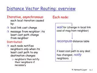
Topic • How to compute shortest paths in a distributed network • The Distance Vector (DV) approach Here’s my vector! Here’s mine CSE 461 University of Washington
Distance Vector Routing • Simple, early routing approach • Used in ARPANET, and “RIP” • One of two main approaches to routing • Distributed version of Bellman-Ford • Works, but very slow convergence after some failures • Link-state algorithms are now typically used in practice • More involved, better behavior CSE 461 University of Washington
Distance Vector Setting Each node computes its forwarding table in a distributed setting: • Nodes know only the cost to their neighbors; not the topology • Nodes can talk only to their neighbors using messages • All nodes run the same algorithm concurrently • Nodes and links may fail, messages may be lost CSE 461 University of Washington
Distance Vector Algorithm Each node maintains a vector of distances to all destinations • Initialize vector with 0 (zero) cost to self, ∞ (infinity) to other destinations • Periodically send vector to neighbors • Update vector for each destination by selecting the shortest distance heard, after adding cost of neighbor link • Use the best neighbor for forwarding CSE 461 University of Washington
Distance Vector (2) F • Consider from the point of view of node A • Can only talk to nodes B and E 2 4 E G 3 10 3 2 D 4 Initial vector 1 A B 4 2 2 H C 3 CSE 461 University of Washington
Distance Vector (3) F • First exchange with B, E; learn best 1-hop routes 2 4 E G 3 10 3 2 D 4 1 A B 4 2 2 H C 3 Learned better route CSE 461 University of Washington
Distance Vector (4) F • Second exchange; learn best 2-hop routes 2 4 E G 3 10 3 2 D 4 1 A B 4 2 2 H C 3 CSE 461 University of Washington
Distance Vector (4) F • Third exchange; learn best 3-hop routes 2 4 E G 3 10 3 2 D 4 1 A B 4 2 2 H C 3 CSE 461 University of Washington
Distance Vector (5) F • Subsequent exchanges; converged 2 4 E G 3 10 3 2 D 4 1 A B 4 2 2 H C 3 CSE 461 University of Washington
Distance Vector Dynamics • Adding routes: • News travels one hop per exchange • Removing routes • When a node fails, no more exchanges, other nodes forget • But partitions (unreachable nodes in divided network) are a problem • “Count to infinity” scenario CSE 461 University of Washington
Dynamics (2) • Good news travels quickly, bad news slowly (inferred) X Desired convergence “Count to infinity” scenario CSE 461 University of Washington
Dynamics (3) • Various heuristics to address • e.g.,“Split horizon, poison reverse” (Don’t send route back to where you learned it from.) • But none are very effective • Link state now favored in practice • Except when very resource-limited CSE 461 University of Washington
Topic • How to compute shortest paths in a distributed network • The Link-State (LS) approach Flood! … then compute CSE 461 University of Washington
Link-State Routing • One of two approaches to routing • Trades more computation than distance vector for better dynamics • Widely used in practice • Used in Internet/ARPANET from 1979 • Modern networks use OSPF and IS-IS CSE 461 University of Washington
Link-State Algorithm Proceeds in two phases: • Nodes flood topology in the form of link state packets • Each node learns full topology • Each node computes its own forwarding table • By running Dijkstra (or equivalent) CSE 461 University of Washington
Topology Dissemination F • Each node floods link state packet (LSP) that describes their portion of the topology 2 4 E G 3 10 3 2 D 4 Node E’s LSP flooded to A, B, C, D, and F 1 A B 4 2 2 H C 3 CSE 461 University of Washington
Route Computation • Each node has full topology • By combining all LSPs • Each node simply runs Dijkstra • Some replicated computation, but finds required routes directly • Compile forwarding table from sink/source tree • That’s it folks! CSE 461 University of Washington
Handling Changes F • Nodes adjacent to failed link or node will notice • Flood updated LSP with less connectivity 2 4 E G 3 10 Failure! F’s LSP B’s LSP 3 2 D 4 1 XXXX A B 4 2 2 H C 3 CSE 461 University of Washington
Handling Changes (2) • Link failure • Both nodes notice, send updated LSPs • Link is removed from topology • Node failure • All neighbors notice a link has failed • Failed node can’t update its own LSP • But it is OK: all links to node removed CSE 461 University of Washington
Handling Changes (3) • Addition of a link or node • Add LSP of new node to topology • Old LSPs are updated with new link • Additions are the easy case … CSE 461 University of Washington
DV/LS Comparison CSE 461 University of Washington
Equal-Cost Multi-Path Routing (§5.2.1)